bundles / scipy 1.17.1 / scipy / fft / _basic / fft
_Function
scipy.fft._basic:fft
source: /scipy/fft/_basic.py :25
Signature
def fft ( x , n = None , axis = -1 , norm = None , overwrite_x = False , workers = None , * , plan = None ) Summary
Compute the 1-D discrete Fourier Transform.
Extended Summary
This function computes the 1-D n-point discrete Fourier Transform (DFT) with the efficient Fast Fourier Transform (FFT) algorithm [1].
Parameters
x: array_likeInput array, can be complex.
n: int, optionalLength of the transformed axis of the output. If
nis smaller than the length of the input, the input is cropped. If it is larger, the input is padded with zeros. Ifnis not given, the length of the input along the axis specified byaxisis used.axis: int, optionalAxis over which to compute the FFT. If not given, the last axis is used.
norm: {"backward", "ortho", "forward"}, optionalNormalization mode. Default is "backward", meaning no normalization on the forward transforms and scaling by
1/non theifft. "forward" instead applies the1/nfactor on the forward transform. Fornorm="ortho", both directions are scaled by1/sqrt(n).overwrite_x: bool, optionalIf True, the contents of
xcan be destroyed; the default is False. See the notes below for more details.workers: int, optionalMaximum number of workers to use for parallel computation. If negative, the value wraps around from
os.cpu_count(). See below for more details.plan: object, optionalThis argument is reserved for passing in a precomputed plan provided by downstream FFT vendors. It is currently not used in SciPy.
Returns
out: complex ndarrayThe truncated or zero-padded input, transformed along the axis indicated by
axis, or the last one ifaxisis not specified.
Raises
: IndexErrorif
axesis larger than the last axis ofx.
Notes
FFT (Fast Fourier Transform) refers to a way the discrete Fourier Transform (DFT) can be calculated efficiently, by using symmetries in the calculated terms. The symmetry is highest when n is a power of 2, and the transform is therefore most efficient for these sizes. For poorly factorizable sizes, scipy.fft uses Bluestein's algorithm [2] and so is never worse than O(n log n). Further performance improvements may be seen by zero-padding the input using next_fast_len.
If x is a 1d array, then the fft is equivalent to
y[k] = np.sum(x * np.exp(-2j * np.pi * k * np.arange(n)/n))The frequency term f=k/n is found at y[k]. At y[n/2] we reach the Nyquist frequency and wrap around to the negative-frequency terms. So, for an 8-point transform, the frequencies of the result are [0, 1, 2, 3, -4, -3, -2, -1]. To rearrange the fft output so that the zero-frequency component is centered, like [-4, -3, -2, -1, 0, 1, 2, 3], use fftshift.
Transforms can be done in single, double, or extended precision (long double) floating point. Half precision inputs will be converted to single precision and non-floating-point inputs will be converted to double precision.
If the data type of x is real, a "real FFT" algorithm is automatically used, which roughly halves the computation time. To increase efficiency a little further, use rfft, which does the same calculation, but only outputs half of the symmetrical spectrum. If the data are both real and symmetrical, the dct can again double the efficiency, by generating half of the spectrum from half of the signal.
When overwrite_x=True is specified, the memory referenced by x may be used by the implementation in any way. This may include reusing the memory for the result, but this is in no way guaranteed. You should not rely on the contents of x after the transform as this may change in future without warning.
The workers argument specifies the maximum number of parallel jobs to split the FFT computation into. This will execute independent 1-D FFTs within x. So, x must be at least 2-D and the non-transformed axes must be large enough to split into chunks. If x is too small, fewer jobs may be used than requested.
Array API Standard Support
fft has experimental support for Python Array API Standard compatible backends in addition to NumPy. Please consider testing these features by setting an environment variable SCIPY_ARRAY_API=1 and providing CuPy, PyTorch, JAX, or Dask arrays as array arguments. The following combinations of backend and device (or other capability) are supported.
====================  ====================  ====================
Library               CPU                   GPU
====================  ====================  ====================
NumPy                 ✅                     n/a
CuPy                  n/a                   ✅
PyTorch               ✅                     ✅
JAX                   ✅                     ✅
Dask                  ⚠️ computes graph     n/a
====================  ====================  ====================
See
dev-arrayapifor more information.
Examples
import scipy.fft
import numpy as np
✓
scipy.fft.fft(np.exp(2j * np.pi * np.arange(8) / 8))
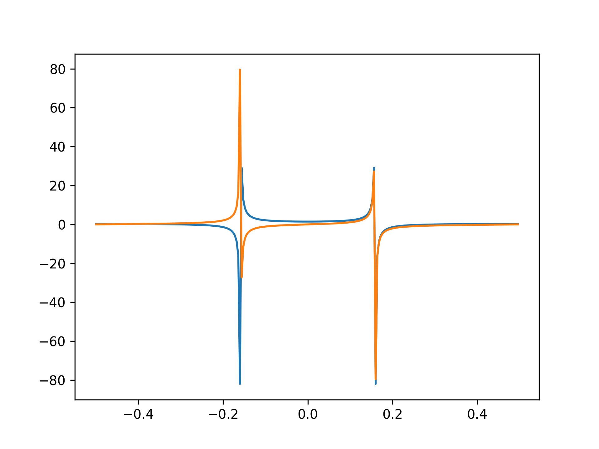
✗from scipy.fft import fft, fftfreq, fftshift import matplotlib.pyplot as plt t = np.arange(256) sp = fftshift(fft(np.sin(t))) freq = fftshift(fftfreq(t.shape[-1]))✓
plt.plot(freq, sp.real, freq, sp.imag)
✗plt.show()
✓
See also
- fft2
The 2-D FFT.
- fftfreq
Frequency bins for given FFT parameters.
- fftn
The N-D FFT.
- ifft
The inverse of
fft.- next_fast_len
Size to pad input to for most efficient transforms
- rfftn
The N-D FFT of real input.
Aliases
-
scipy.fft.fft
Referenced by
This package
- tutorial:parallel_execution
- scipy.fft._basic:fft2
- scipy.fft._basic:fftn
- scipy.fft._basic:hfft
- scipy.fft._basic:hfft2
- scipy.fft._basic:hfftn
- scipy.fft._basic:ifft
- scipy.fft._basic:ifft2
- scipy.fft._basic:ifftn
- scipy.fft._basic:ihfft
- scipy.fft._basic:ihfft2
- scipy.fft._basic:ihfftn
- scipy.fft._basic:irfft
- scipy.fft._basic:irfft2
- scipy.fft._basic:irfftn
- scipy.fft._basic:rfft
- scipy.fft._basic:rfft2
- scipy.fft._basic:rfftn
- scipy.fft._realtransforms:dct
- scipy.fft._realtransforms:dctn
- scipy.fft._realtransforms:dst
- scipy.fft._realtransforms:dstn
- scipy.fft._realtransforms:idct
- scipy.fft._realtransforms:idctn
- scipy.fft._realtransforms:idst
- scipy.fft._realtransforms:idstn
- scipy.linalg._special_matrices:dft
- scipy.signal._short_time_fft:ShortTimeFFT.from_win_equals_dual
- scipy.signal._signaltools:resample