`scipy.interpolate._dierckx:evaluate_all_bspl`

Summary

Evaluate the k+1 B-splines which are non-zero on interval m.

Parameters

t : ndarray, shape (nt + k + 1,): sorted 1D array of knots
k : int: spline order
xval: float: argument at which to evaluate the B-splines
m : int: index of the left edge of the evaluation interval, t[m] <= x < t[m+1]
nu : int, optional: Evaluate derivatives order nu. Default is zero.

Returns

: ndarray, shape (k+1,): The values of B-splines $[B_{m - k} (xv a l), ..., B_{m} (xv a l)]$ if nu is zero, otherwise the derivatives of order nu.

Examples

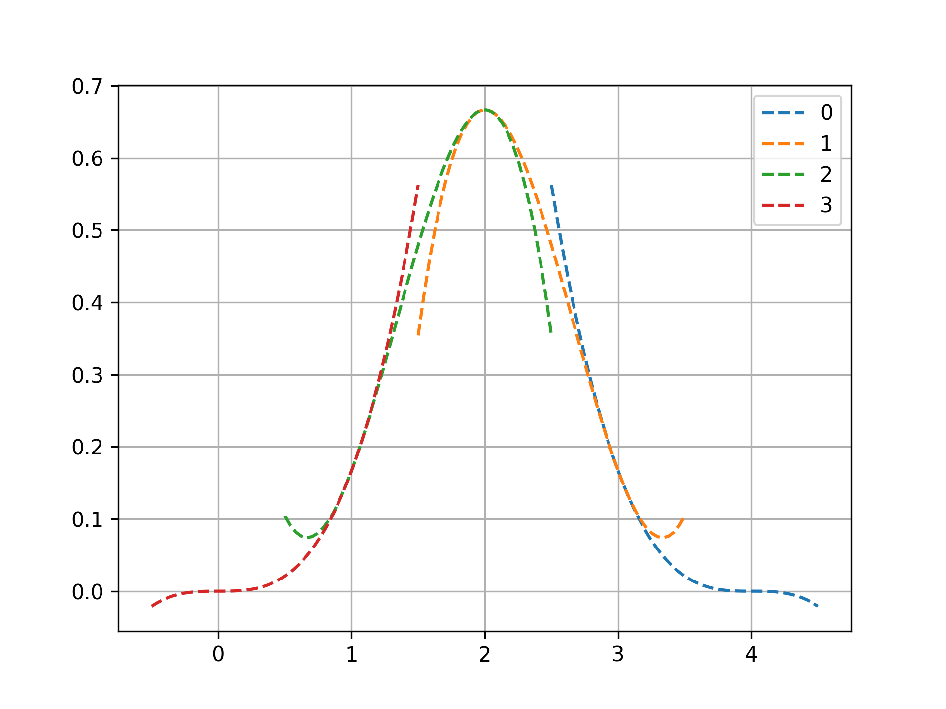
A textbook use of this sort of routine is plotting the ``k+1`` polynomial pieces which make up a B-spline of order `k`. Consider a cubic spline

k = 3 
t = [0., 1., 2., 3., 4.]   # internal knots 
a, b = t[0], t[-1]    # base interval is [a, b) 
t = np.array([a]*k + t + [b]*k)  # add boundary knots

✓

import matplotlib.pyplot as plt 
xx = np.linspace(a, b, 100)

✓

plt.plot(xx, BSpline.basis_element(t[k:-k])(xx), 
         lw=3, alpha=0.5, label='basis_element')

⚠

Now we use slide an interval ``t[m]..t[m+1]`` along the base interval ``a..b`` and use `evaluate_all_bspl` to compute the restriction of the B-spline of interest to this interval:

for i in range(k+1): 
   x1, x2 = t[2*k - i], t[2*k - i + 1] 
   xx = np.linspace(x1 - 0.5, x2 + 0.5) 
   yy = [evaluate_all_bspl(t, k, x, 2*k - i)[i] for x in xx] 
   plt.plot(xx, yy, '--', label=str(i))

✗

plt.grid(True)

✓

plt.legend()

✗

plt.show()

✓

Aliases

scipy.interpolate._dierckx.evaluate_all_bspl