`scipy.interpolate._fitpack2:SphereBivariateSpline.call`

source: /scipy/interpolate/_fitpack2.py :1699

Signature

   def     __call__ (    self    ,    theta    ,    phi    ,    dtheta    =  0   ,    dphi    =  0   ,    grid    =  True     )

Summary

Evaluate the spline or its derivatives at given positions.

Parameters

theta, phi : array_like

Input coordinates.

If grid is False, evaluate the spline at points (theta[i], phi[i]), i=0, ..., len(x)-1. Standard Numpy broadcasting is obeyed.

If grid is True: evaluate spline at the grid points defined by the coordinate arrays theta, phi. The arrays must be sorted to increasing order. The ordering of axes is consistent with np.meshgrid(..., indexing="ij") and inconsistent with the default ordering np.meshgrid(..., indexing="xy").

dtheta : int, optional

Order of theta-derivative

dphi : int

Order of phi-derivative

grid : bool

Whether to evaluate the results on a grid spanned by the input arrays, or at points specified by the input arrays.

Examples

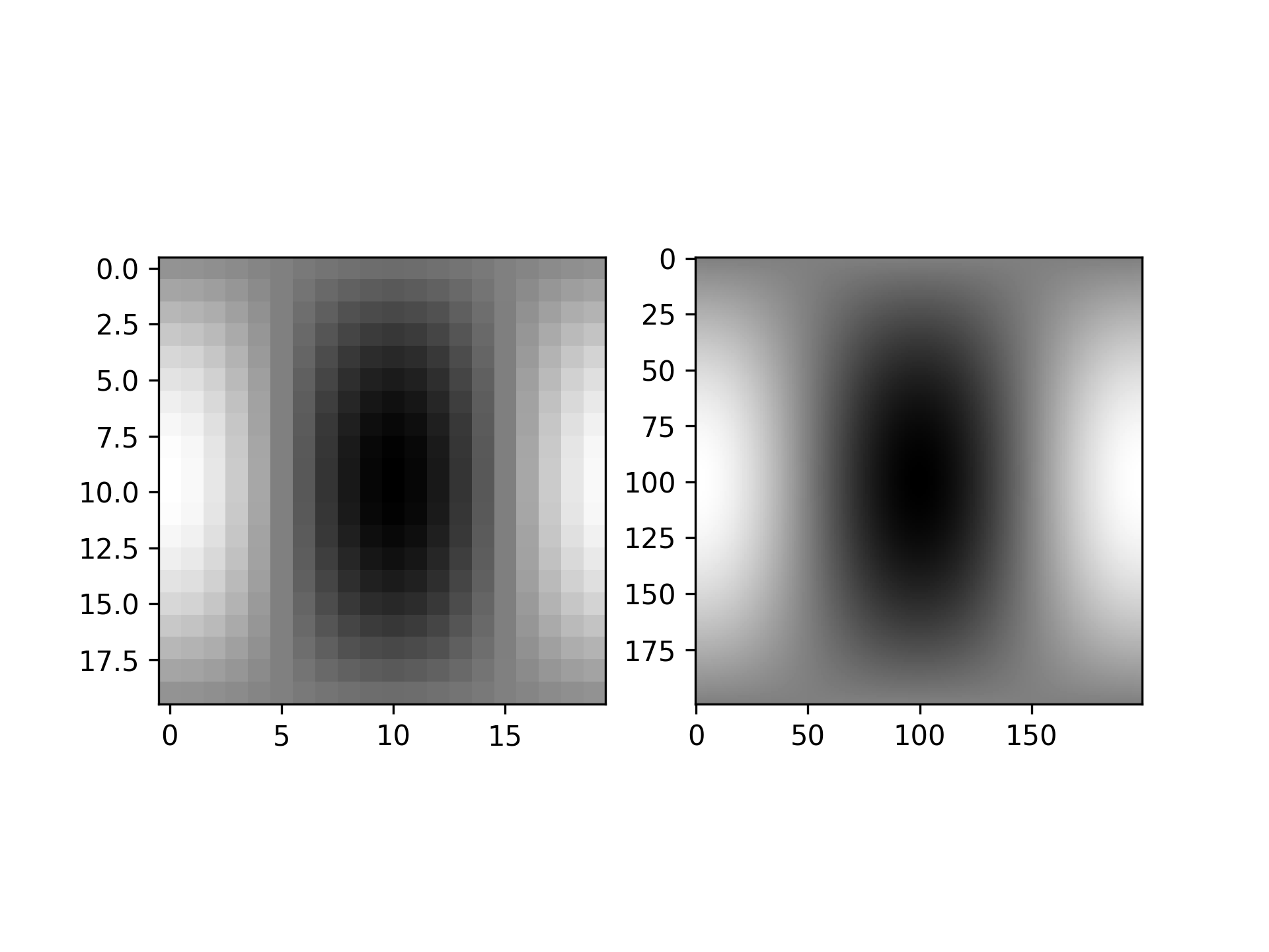
Suppose that we want to use splines to interpolate a bivariate function on a sphere. The value of the function is known on a grid of longitudes and colatitudes.

import numpy as np
from scipy.interpolate import RectSphereBivariateSpline
def f(theta, phi):
    return np.sin(theta) * np.cos(phi)

✓

We evaluate the function on the grid. Note that the default indexing="xy" of meshgrid would result in an unexpected (transposed) result after interpolation.

thetaarr = np.linspace(0, np.pi, 22)[1:-1]
phiarr = np.linspace(0, 2 * np.pi, 21)[:-1]
thetagrid, phigrid = np.meshgrid(thetaarr, phiarr, indexing="ij")
zdata = f(thetagrid, phigrid)

✓

We next set up the interpolator and use it to evaluate the function on a finer grid.

rsbs = RectSphereBivariateSpline(thetaarr, phiarr, zdata)
thetaarr_fine = np.linspace(0, np.pi, 200)
phiarr_fine = np.linspace(0, 2 * np.pi, 200)
zdata_fine = rsbs(thetaarr_fine, phiarr_fine)

✓

Finally we plot the coarsly-sampled input data alongside the finely-sampled interpolated data to check that they agree.

import matplotlib.pyplot as plt
fig = plt.figure()
ax1 = fig.add_subplot(1, 2, 1)
ax2 = fig.add_subplot(1, 2, 2)

✓

ax1.imshow(zdata)
ax2.imshow(zdata_fine)

✗

plt.show()

✓

Aliases

scipy.interpolate._fitpack2.SphereBivariateSpline.__call__