`scipy.interpolate._fitpack2:_BivariateSplineBase.call`

source: /scipy/interpolate/_fitpack2.py :978

Signature

   def     __call__ (    self    ,    x    ,    y    ,    dx    =  0   ,    dy    =  0   ,    grid    =  True     )

Summary

Evaluate the spline or its derivatives at given positions.

Parameters

x, y : array_like

Input coordinates.

If grid is False, evaluate the spline at points (x[i], y[i]), i=0, ..., len(x)-1. Standard Numpy broadcasting is obeyed.

If grid is True: evaluate spline at the grid points defined by the coordinate arrays x, y. The arrays must be sorted to increasing order.

The ordering of axes is consistent with np.meshgrid(..., indexing="ij") and inconsistent with the default ordering np.meshgrid(..., indexing="xy").

dx : int

Order of x-derivative

dy : int

Order of y-derivative

grid : bool

Whether to evaluate the results on a grid spanned by the input arrays, or at points specified by the input arrays.

Examples

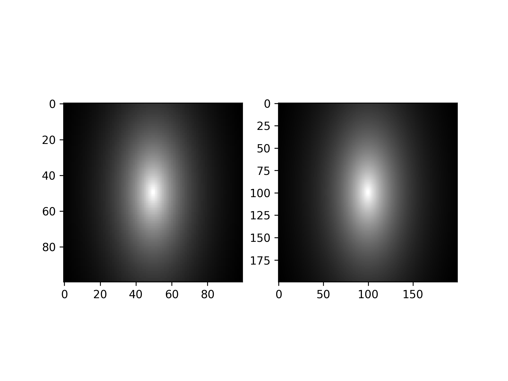
Suppose that we want to bilinearly interpolate an exponentially decaying function in 2 dimensions.

import numpy as np
from scipy.interpolate import RectBivariateSpline

✓

We sample the function on a coarse grid. Note that the default indexing="xy" of meshgrid would result in an unexpected (transposed) result after interpolation.

xarr = np.linspace(-3, 3, 100)
yarr = np.linspace(-3, 3, 100)
xgrid, ygrid = np.meshgrid(xarr, yarr, indexing="ij")

✓

The function to interpolate decays faster along one axis than the other.

zdata = np.exp(-np.sqrt((xgrid / 2) ** 2 + ygrid**2))

✓

Next we sample on a finer grid using interpolation (kx=ky=1 for bilinear).

rbs = RectBivariateSpline(xarr, yarr, zdata, kx=1, ky=1)
xarr_fine = np.linspace(-3, 3, 200)
yarr_fine = np.linspace(-3, 3, 200)
xgrid_fine, ygrid_fine = np.meshgrid(xarr_fine, yarr_fine, indexing="ij")
zdata_interp = rbs(xgrid_fine, ygrid_fine, grid=False)

✓

And check that the result agrees with the input by plotting both.

import matplotlib.pyplot as plt
fig = plt.figure()
ax1 = fig.add_subplot(1, 2, 1, aspect="equal")
ax2 = fig.add_subplot(1, 2, 2, aspect="equal")

✓

ax1.imshow(zdata)
ax2.imshow(zdata_interp)

✗

plt.show()

✓

Aliases

scipy.interpolate._fitpack2._BivariateSplineBase.__call__