`scipy.interpolate._interpolate:lagrange`

source: /scipy/interpolate/_interpolate.py :22

Signature

def lagrange ( x , w )

Summary

Return a Lagrange interpolating polynomial.

Extended Summary

Given two 1-D arrays x and w, returns the Lagrange interpolating polynomial through the points (x, w).

Warning: This implementation is numerically unstable. Do not expect to be able to use more than about 20 points even if they are chosen optimally.

Parameters

x : array_like: x represents the x-coordinates of a set of datapoints.
w : array_like: w represents the y-coordinates of a set of datapoints, i.e., f(x).

Returns

lagrange : `numpy.poly1d` instance: The Lagrange interpolating polynomial.

Notes

The name of this function refers to the fact that the returned object represents a Lagrange polynomial, the unique polynomial of lowest degree that interpolates a given set of data ^[1]. It computes the polynomial using Newton's divided differences formula ^[2]; that is, it works with Newton basis polynomials rather than Lagrange basis polynomials. For numerical calculations, the barycentric form of Lagrange interpolation (scipy.interpolate.BarycentricInterpolator) is typically more appropriate.

Examples

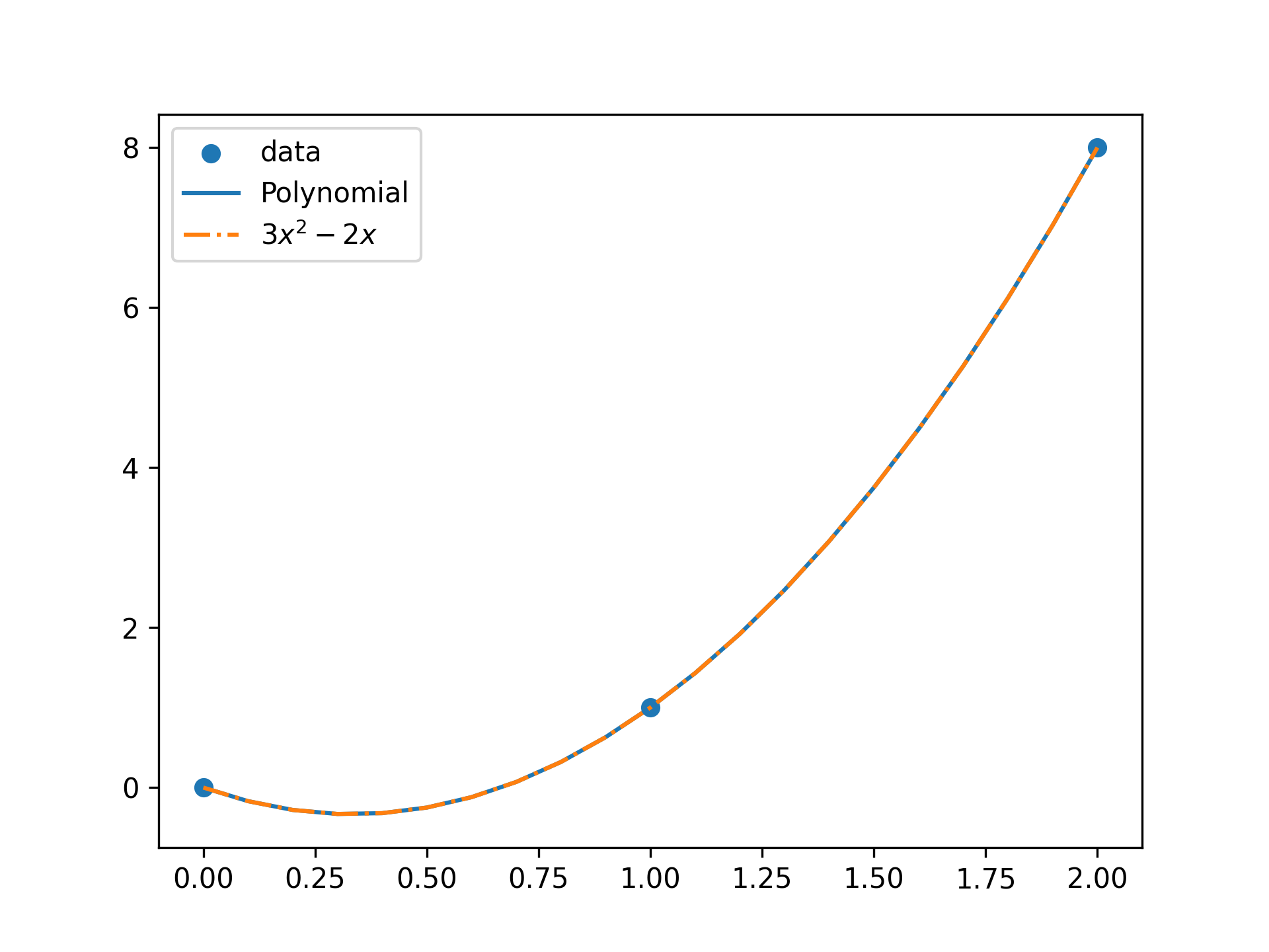
Interpolate :math:`f(x) = x^3` by 3 points.

import numpy as np
from scipy.interpolate import lagrange
x = np.array([0, 1, 2])
y = x**3
poly = lagrange(x, y)

✓

Since there are only 3 points, the Lagrange polynomial has degree 2. Explicitly, it is given by .. math:: \begin{aligned} L(x) &= 1\times \frac{x (x - 2)}{-1} + 8\times \frac{x (x-1)}{2} \\ &= x (-2 + 3x) \end{aligned}

from numpy.polynomial.polynomial import Polynomial
Polynomial(poly.coef[::-1]).coef

✓

import matplotlib.pyplot as plt
x_new = np.arange(0, 2.1, 0.1)

✓

plt.scatter(x, y, label='data')
plt.plot(x_new, Polynomial(poly.coef[::-1])(x_new), label='Polynomial')
plt.plot(x_new, 3*x_new**2 - 2*x_new + 0*x_new,
         label=r"$3 x^2 - 2 x$", linestyle='-.')
plt.legend()

✗

plt.show()

✓

Aliases

scipy.interpolate.lagrange