bundles / scipy 1.17.1 / scipy / optimize / _minpack_py / curve_fit
function
scipy.optimize._minpack_py:curve_fit
Signature
def curve_fit ( f , xdata , ydata , p0 = None , sigma = None , absolute_sigma = False , check_finite = None , bounds = (-inf, inf) , method = None , jac = None , * , full_output = False , nan_policy = None , ** kwargs ) Summary
Use non-linear least squares to fit a function, f, to data.
Extended Summary
Assumes ydata = f(xdata, *params) + eps.
Parameters
f: callableThe model function, f(x, ...). It must take the independent variable as the first argument and the parameters to fit as separate remaining arguments.
xdata: array_likeThe independent variable where the data is measured. Should usually be an M-length sequence or an (k,M)-shaped array for functions with k predictors, and each element should be float convertible if it is an array like object.
ydata: array_likeThe dependent data, a length M array - nominally
f(xdata, ...).p0: array_like, optionalInitial guess for the parameters (length N). If None, then the initial values will all be 1 (if the number of parameters for the function can be determined using introspection, otherwise a ValueError is raised).
sigma: None or scalar or M-length sequence or MxM array, optionalDetermines the uncertainty in
ydata. If we define residuals asr = ydata - f(xdata, *popt), then the interpretation ofsigmadepends on its number of dimensions:A scalar or 1-D
sigmashould contain values of standard deviations of errors inydata. In this case, the optimized function ischisq = sum((r / sigma) ** 2).A 2-D
sigmashould contain the covariance matrix of errors inydata. In this case, the optimized function ischisq = r.T @ inv(sigma) @ r.
None (default) is equivalent of 1-D
sigmafilled with ones.absolute_sigma: bool, optionalIf True,
sigmais used in an absolute sense and the estimated parameter covariance pcov reflects these absolute values.If False (default), only the relative magnitudes of the
sigmavalues matter. The returned parameter covariance matrix pcov is based on scalingsigmaby a constant factor. This constant is set by demanding that the reducedchisqfor the optimal parameters popt when using the scaledsigmaequals unity. In other words,sigmais scaled to match the sample variance of the residuals after the fit. Default is False. Mathematically,pcov(absolute_sigma=False) = pcov(absolute_sigma=True) * chisq(popt)/(M-N)check_finite: bool, optionalIf True, check that the input arrays do not contain nans of infs, and raise a ValueError if they do. Setting this parameter to False may silently produce nonsensical results if the input arrays do contain nans. Default is True if
nan_policyis not specified explicitly and False otherwise.bounds: 2-tuple of array_like or `Bounds`, optionalLower and upper bounds on parameters. Defaults to no bounds. There are two ways to specify the bounds:
Instance of Bounds class.
2-tuple of array_like: Each element of the tuple must be either an array with the length equal to the number of parameters, or a scalar (in which case the bound is taken to be the same for all parameters). Use
np.infwith an appropriate sign to disable bounds on all or some parameters.
method: {'lm', 'trf', 'dogbox'}, optionalMethod to use for optimization. See least_squares for more details. Default is 'lm' for unconstrained problems and 'trf' if
boundsare provided. The method 'lm' won't work when the number of observations is less than the number of variables, use 'trf' or 'dogbox' in this case.jac: callable, string or None, optionalFunction with signature
jac(x, ...)which computes the Jacobian matrix of the model function with respect to parameters as a dense array_like structure. It will be scaled according to providedsigma. If None (default), the Jacobian will be estimated numerically. String keywords for 'trf' and 'dogbox' methods can be used to select a finite difference scheme, see least_squares.full_output: boolean, optionalIf True, this function returns additional information: infodict, mesg, and ier.
nan_policy: {'raise', 'omit', None}, optionalDefines how to handle when input contains nan. The following options are available (default is None):
'raise': throws an error
'omit': performs the calculations ignoring nan values
None: no special handling of NaNs is performed (except what is done by check_finite); the behavior when NaNs are present is implementation-dependent and may change.
Note that if this value is specified explicitly (not None),
check_finitewill be set as False.**kwargsKeyword arguments passed to leastsq for
method='lm'or least_squares otherwise.
Returns
popt: arrayOptimal values for the parameters so that the sum of the squared residuals of
f(xdata, *popt) - ydatais minimized.pcov: 2-D arrayThe estimated approximate covariance of popt. The diagonals provide the variance of the parameter estimate. To compute one standard deviation errors on the parameters, use
perr = np.sqrt(np.diag(pcov)). Note that the relationship betweencovand parameter error estimates is derived based on a linear approximation to the model function around the optimum [1]. When this approximation becomes inaccurate,covmay not provide an accurate measure of uncertainty.How the
sigmaparameter affects the estimated covariance depends onabsolute_sigmaargument, as described above.If the Jacobian matrix at the solution doesn't have a full rank, then 'lm' method returns a matrix filled with
np.inf, on the other hand 'trf' and 'dogbox' methods use Moore-Penrose pseudoinverse to compute the covariance matrix. Covariance matrices with large condition numbers (e.g. computed with numpy.linalg.cond) may indicate that results are unreliable.infodict: dict (returned only if `full_output` is True)a dictionary of optional outputs with the keys:
nfevThe number of function calls. Methods 'trf' and 'dogbox' do not count function calls for numerical Jacobian approximation, as opposed to 'lm' method.
fvecThe residual values evaluated at the solution, for a 1-D
sigmathis is(f(x, *popt) - ydata)/sigma.fjacA permutation of the R matrix of a QR factorization of the final approximate Jacobian matrix, stored column wise. Together with ipvt, the covariance of the estimate can be approximated. Method 'lm' only provides this information.
ipvtAn integer array of length N which defines a permutation matrix, p, such that fjac*p = q*r, where r is upper triangular with diagonal elements of nonincreasing magnitude. Column j of p is column ipvt(j) of the identity matrix. Method 'lm' only provides this information.
qtfThe vector (transpose(q) * fvec). Method 'lm' only provides this information.
mesg: str (returned only if `full_output` is True)A string message giving information about the solution.
ier: int (returned only if `full_output` is True)An integer flag. If it is equal to 1, 2, 3 or 4, the solution was found. Otherwise, the solution was not found. In either case, the optional output variable mesg gives more information.
Raises
: ValueErrorif either
ydataorxdatacontain NaNs, or if incompatible options are used.: RuntimeErrorif the least-squares minimization fails.
: OptimizeWarningif covariance of the parameters can not be estimated.
Notes
Users should ensure that inputs xdata, ydata, and the output of f are float64, or else the optimization may return incorrect results.
With method='lm', the algorithm uses the Levenberg-Marquardt algorithm through leastsq. Note that this algorithm can only deal with unconstrained problems.
Box constraints can be handled by methods 'trf' and 'dogbox'. Refer to the docstring of least_squares for more information.
Parameters to be fitted must have similar scale. Differences of multiple orders of magnitude can lead to incorrect results. For the 'trf' and 'dogbox' methods, the x_scale keyword argument can be used to scale the parameters.
curve_fit is for local optimization of parameters to minimize the sum of squares of residuals. For global optimization, other choices of objective function, and other advanced features, consider using SciPy's tutorial_optimize_global tools or the LMFIT package.
Examples
import numpy as np
import matplotlib.pyplot as plt
from scipy.optimize import curve_fit
✓
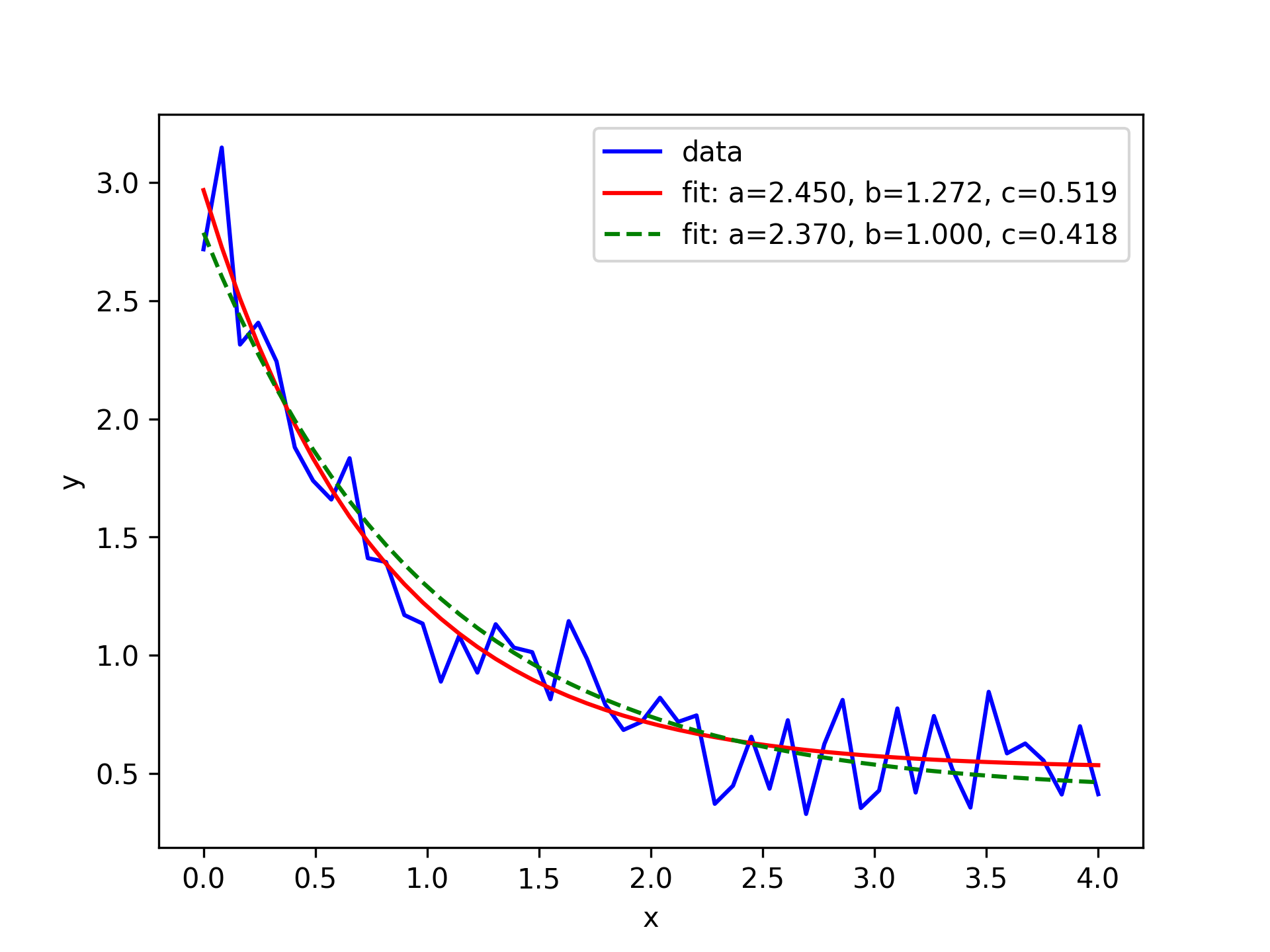
def func(x, a, b, c):
    return a * np.exp(-b * x) + c
✓
xdata = np.linspace(0, 4, 50)
y = func(xdata, 2.5, 1.3, 0.5)
rng = np.random.default_rng()
y_noise = 0.2 * rng.normal(size=xdata.size)
ydata = y + y_noise
✓
plt.plot(xdata, ydata, 'b-', label='data')
✗popt, pcov = curve_fit(func, xdata, ydata)
✓popt plt.plot(xdata, func(xdata, *popt), 'r-', label='fit: a=%5.3f, b=%5.3f, c=%5.3f' % tuple(popt))✗
popt, pcov = curve_fit(func, xdata, ydata, bounds=(0, [3., 1., 0.5]))
✓popt plt.plot(xdata, func(xdata, *popt), 'g--', label='fit: a=%5.3f, b=%5.3f, c=%5.3f' % tuple(popt))✗
plt.xlabel('x')
plt.ylabel('y')
plt.legend()
✗
plt.show()
✓
np.linalg.cond(pcov)
✗def func2(x, a, b, c, d): return a * d * np.exp(-b * x) + c # a and d are redundant popt, pcov = curve_fit(func2, xdata, ydata)✓
np.linalg.cond(pcov)
✗np.diag(pcov)
✗ydata = func(xdata, 500000, 0.01, 15)
✓try: popt, pcov = curve_fit(func, xdata, ydata, method = 'trf') except RuntimeError as e: print(e)✗
popt, pcov = curve_fit(func, xdata, ydata, method = 'trf',
                       x_scale = [1000, 1, 1])
✓
popt
✗See also
- least_squares
Minimize the sum of squares of nonlinear functions.
- scipy.stats.linregress
Calculate a linear least squares regression for two sets of measurements.
Aliases
-
scipy.optimize.curve_fit