`scipy.signal.windows._windows:dpss`

source: /scipy/signal/windows/_windows.py :1970

Signature

   def     dpss (    M    ,    NW    ,    Kmax    =  None   ,    sym    =  True   ,    norm    =  None   ,    return_ratios    =  False   ,  * ,     xp    =  None   ,    device    =  None     )

Summary

Compute the Discrete Prolate Spheroidal Sequences (DPSS).

Extended Summary

DPSS (or Slepian sequences) are often used in multitaper power spectral density estimation (see ^[1]). The first window in the sequence can be used to maximize the energy concentration in the main lobe, and is also called the Slepian window.

Parameters

M : int: Window length.
NW : float: Standardized half bandwidth corresponding to 2*NW = BW/f0 = BW*M*dt where dt is taken as 1.
Kmax : int | None, optional: Number of DPSS windows to return (orders 0 through Kmax-1). If None (default), return only a single window of shape (M,) instead of an array of windows of shape (Kmax, M).
sym : bool, optional: When True (default), generates a symmetric window, for use in filter design. When False, generates a periodic window, for use in spectral analysis.
norm : {2, 'approximate', 'subsample'} | None, optional: If 'approximate' or 'subsample', then the windows are normalized by the maximum, and a correction scale-factor for even-length windows is applied either using M**2/(M**2+NW) ("approximate") or a FFT-based subsample shift ("subsample"), see Notes for details. If None, then "approximate" is used when Kmax=None and 2 otherwise (which uses the l2 norm).
return_ratios : bool, optional: If True, also return the concentration ratios in addition to the windows.
xp : array_namespace, optional: Optional array namespace. Should be compatible with the array API standard, or supported by array-api-compat. Default: numpy
device: any: optional device specification for output. Should match one of the supported device specification in xp.

Returns

v : ndarray, shape (Kmax, M) or (M,): The DPSS windows. Will be 1D if Kmax is None.
r : ndarray, shape (Kmax,) or float, optional: The concentration ratios for the windows. Only returned if return_ratios evaluates to True. Will be 0D if Kmax is None.

Notes

This computation uses the tridiagonal eigenvector formulation given in ^[2].

The default normalization for Kmax=None, i.e. window-generation mode, simply using the l-infinity norm would create a window with two unity values, which creates slight normalization differences between even and odd orders. The approximate correction of M**2/float(M**2+NW) for even sample numbers is used to counteract this effect (see Examples below).

For very long signals (e.g., 1e6 elements), it can be useful to compute windows orders of magnitude shorter and use interpolation (e.g., scipy.interpolate.interp1d) to obtain tapers of length M, but this in general will not preserve orthogonality between the tapers.

Array API Standard Support

dpss has experimental support for Python Array API Standard compatible backends in addition to NumPy. Please consider testing these features by setting an environment variable SCIPY_ARRAY_API=1 and providing CuPy, PyTorch, JAX, or Dask arrays as array arguments. The following combinations of backend and device (or other capability) are supported.

====================  ====================  ====================
Library               CPU                   GPU
====================  ====================  ====================
NumPy                 ✅                     n/a                 
CuPy                  n/a                   ⛔                   
PyTorch               ⛔                     ⛔                   
JAX                   ⛔                     ⛔                   
Dask                  ⛔                     n/a                 
====================  ====================  ====================

See dev-arrayapi for more information.

Examples

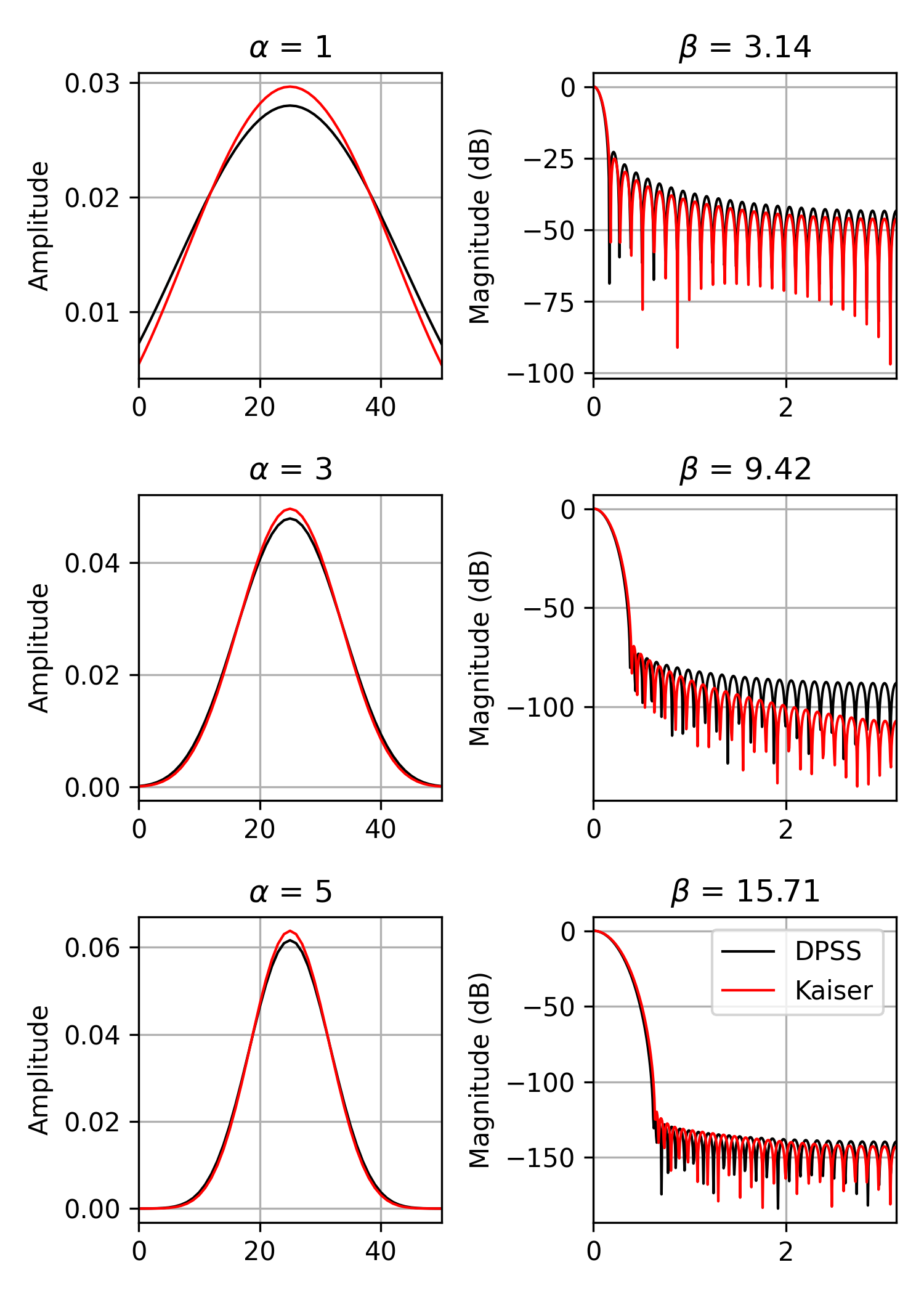
We can compare the window to `kaiser`, which was invented as an alternative that was easier to calculate [3]_ (example adapted from `here <https://ccrma.stanford.edu/~jos/sasp/Kaiser_DPSS_Windows_Compared.html>`_):

import numpy as np
import matplotlib.pyplot as plt
from scipy.signal import windows, freqz
M = 51
fig, axes = plt.subplots(3, 2, figsize=(5, 7))

✓

for ai, alpha in enumerate((1, 3, 5)):
    win_dpss = windows.dpss(M, alpha)
    beta = alpha*np.pi
    win_kaiser = windows.kaiser(M, beta)
    for win, c in ((win_dpss, 'k'), (win_kaiser, 'r')):
        win /= win.sum()
        axes[ai, 0].plot(win, color=c, lw=1.)
        axes[ai, 0].set(xlim=[0, M-1], title=rf'$\alpha$ = {alpha}',
                        ylabel='Amplitude')
        w, h = freqz(win)
        axes[ai, 1].plot(w, 20 * np.log10(np.abs(h)), color=c, lw=1.)
        axes[ai, 1].set(xlim=[0, np.pi],
                        title=rf'$\beta$ = {beta:0.2f}',
                        ylabel='Magnitude (dB)')

✗

for ax in axes.ravel():
    ax.grid(True)

✓

axes[2, 1].legend(['DPSS', 'Kaiser'])

✗

fig.tight_layout()
plt.show()

✓

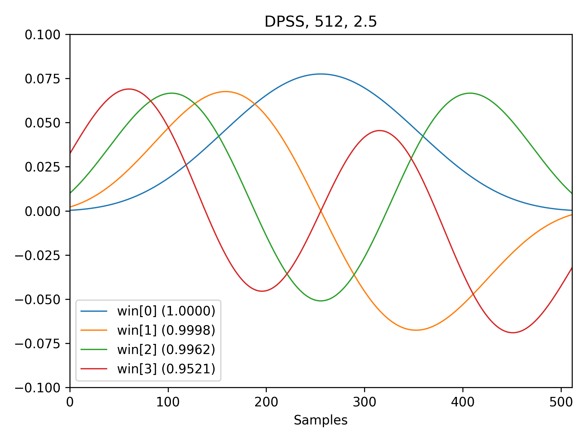
And here are examples of the first four windows, along with their concentration ratios:

M = 512
NW = 2.5
win, eigvals = windows.dpss(M, NW, 4, return_ratios=True)
fig, ax = plt.subplots(1)

✓

ax.plot(win.T, linewidth=1.)
ax.set(xlim=[0, M-1], ylim=[-0.1, 0.1], xlabel='Samples',
       title=f'DPSS, {M:d}, {NW:0.1f}')
ax.legend([f'win[{ii}] ({ratio:0.4f})'
           for ii, ratio in enumerate(eigvals)])

✗

fig.tight_layout()
plt.show()

✓

Using a standard :math:`l_{\infty}` norm would produce two unity values for even `M`, but only one unity value for odd `M`. This produces uneven window power that can be counteracted by the approximate correction ``M**2/float(M**2+NW)``, which can be selected by using ``norm='approximate'`` (which is the same as ``norm=None`` when ``Kmax=None``, as is the case here). Alternatively, the slower ``norm='subsample'`` can be used, which uses subsample shifting in the frequency domain (FFT) to compute the correction:

Ms = np.arange(1, 41)
factors = (50, 20, 10, 5, 2.0001)
energy = np.empty((3, len(Ms), len(factors)))
for mi, M in enumerate(Ms):
    for fi, factor in enumerate(factors):
        NW = M / float(factor)
        # Corrected using empirical approximation (default)
        win = windows.dpss(M, NW)
        energy[0, mi, fi] = np.sum(win ** 2) / np.sqrt(M)
        # Corrected using subsample shifting
        win = windows.dpss(M, NW, norm='subsample')
        energy[1, mi, fi] = np.sum(win ** 2) / np.sqrt(M)
        # Uncorrected (using l-infinity norm)
        win /= win.max()
        energy[2, mi, fi] = np.sum(win ** 2) / np.sqrt(M)
fig, ax = plt.subplots(1)
hs = ax.plot(Ms, energy[2], '-o', markersize=4,
             markeredgecolor='none')
leg = [hs[-1]]
for hi, hh in enumerate(hs):
    h1 = ax.plot(Ms, energy[0, :, hi], '-o', markersize=4,
                 color=hh.get_color(), markeredgecolor='none',
                 alpha=0.66)
    h2 = ax.plot(Ms, energy[1, :, hi], '-o', markersize=4,
                 color=hh.get_color(), markeredgecolor='none',
                 alpha=0.33)
    if hi == len(hs) - 1:
        leg.insert(0, h1[0])
        leg.insert(0, h2[0])

✓

ax.set(xlabel='M (samples)', ylabel=r'Power / $\sqrt{M}$')
ax.legend(leg, ['Uncorrected', r'Corrected: $\frac{M^2}{M^2+NW}$',
                'Corrected (subsample)'])

✗

fig.tight_layout()

✓

Aliases

scipy.signal.windows.dpss

Referenced by

This package

release:1.1.0-notes