`scipy.special._orthogonal:genlaguerre`

source: /scipy/special/_orthogonal.py :586

Signature

def genlaguerre ( n , alpha , monic = False )

Summary

Generalized (associated) Laguerre polynomial.

Extended Summary

Defined to be the solution of

x \frac{d ^{2}}{d x ^{2}} L_{n}^{(α)} + (α + 1 - x) \frac{d}{d x} L_{n}^{(α)} + n L_{n}^{(α)} = 0,

where $α > - 1$ ; $L_{n}^{(α)}$ is a polynomial of degree $n$ .

Parameters

n : int: Degree of the polynomial.
alpha : float: Parameter, must be greater than -1.
monic : bool, optional: If True, scale the leading coefficient to be 1. Default is False.

Returns

L : orthopoly1d: Generalized Laguerre polynomial.

Notes

For fixed $α$ , the polynomials $L_{n}^{(α)}$ are orthogonal over $[0, \infty)$ with weight function $e^{- x} x^{α}$ .

The Laguerre polynomials are the special case where $α = 0$ .

Examples

The generalized Laguerre polynomials are closely related to the confluent hypergeometric function :math:`{}_1F_1`: .. math:: L_n^{(\alpha)} = \binom{n + \alpha}{n} {}_1F_1(-n, \alpha +1, x) This can be verified, for example, for :math:`n = \alpha = 3` over the interval :math:`[-1, 1]`:

import numpy as np
from scipy.special import binom
from scipy.special import genlaguerre
from scipy.special import hyp1f1
x = np.arange(-1.0, 1.0, 0.01)
np.allclose(genlaguerre(3, 3)(x), binom(6, 3) * hyp1f1(-3, 4, x))

✓

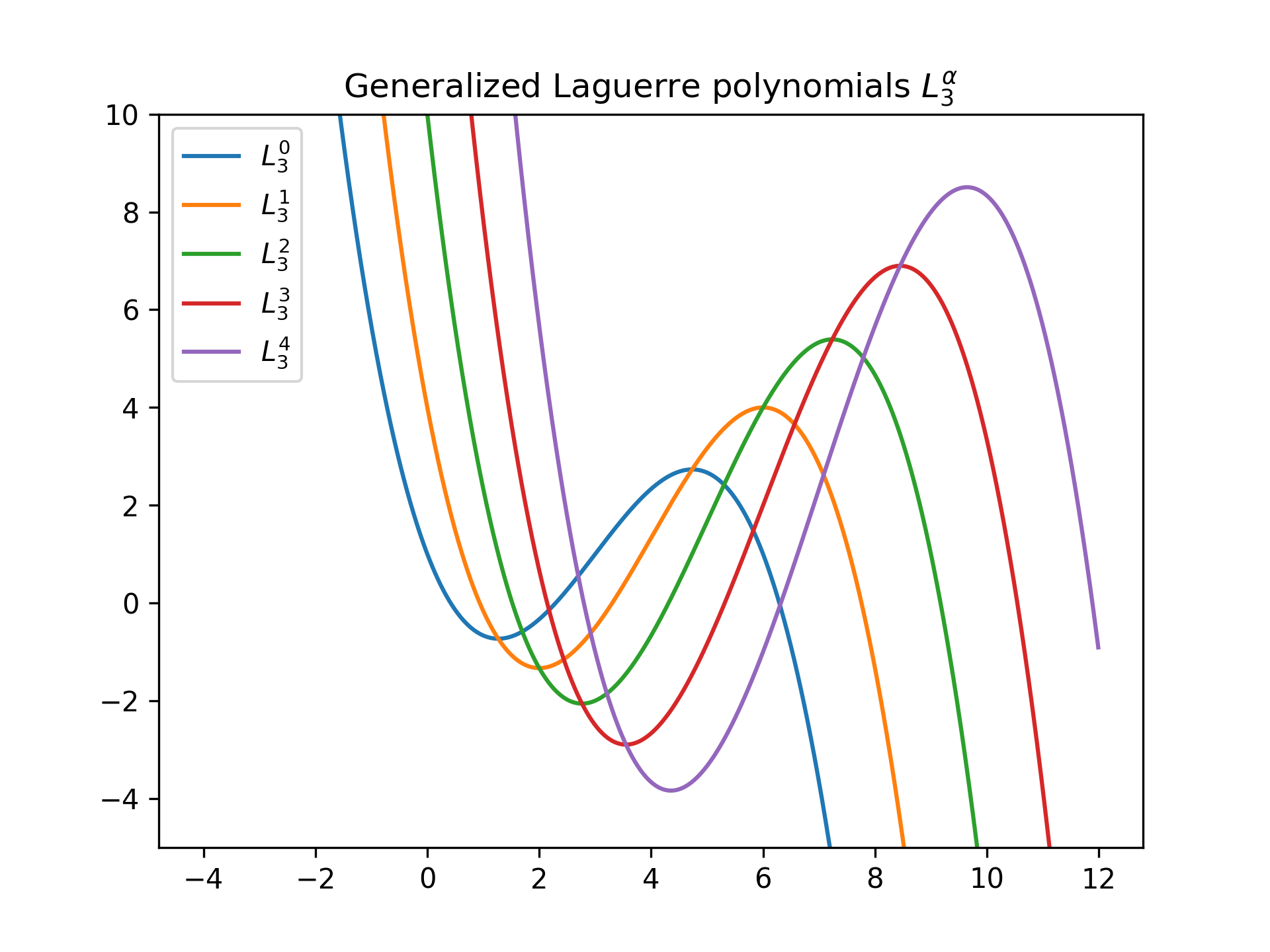
This is the plot of the generalized Laguerre polynomials :math:`L_3^{(\alpha)}` for some values of :math:`\alpha`:

import matplotlib.pyplot as plt
x = np.arange(-4.0, 12.0, 0.01)
fig, ax = plt.subplots()

✓

ax.set_ylim(-5.0, 10.0)
ax.set_title(r'Generalized Laguerre polynomials $L_3^{\alpha}$')
for alpha in np.arange(0, 5):
    ax.plot(x, genlaguerre(3, alpha)(x), label=rf'$L_3^{(alpha)}$')
plt.legend(loc='best')

✗

plt.show()

✓

Aliases

scipy.special.genlaguerre