`scipy.stats._discrete_distns:randint_gen`

source: /scipy/stats/_discrete_distns.py :1177

Signature

   class     randint_gen (    a    =  0   ,    b    =  inf   ,    name    =  None   ,    badvalue    =  None   ,    moment_tol    =  1e-08   ,    values    =  None   ,    inc    =  1   ,    longname    =  None   ,    shapes    =  None   ,    seed    =  None     )

Members

Summary

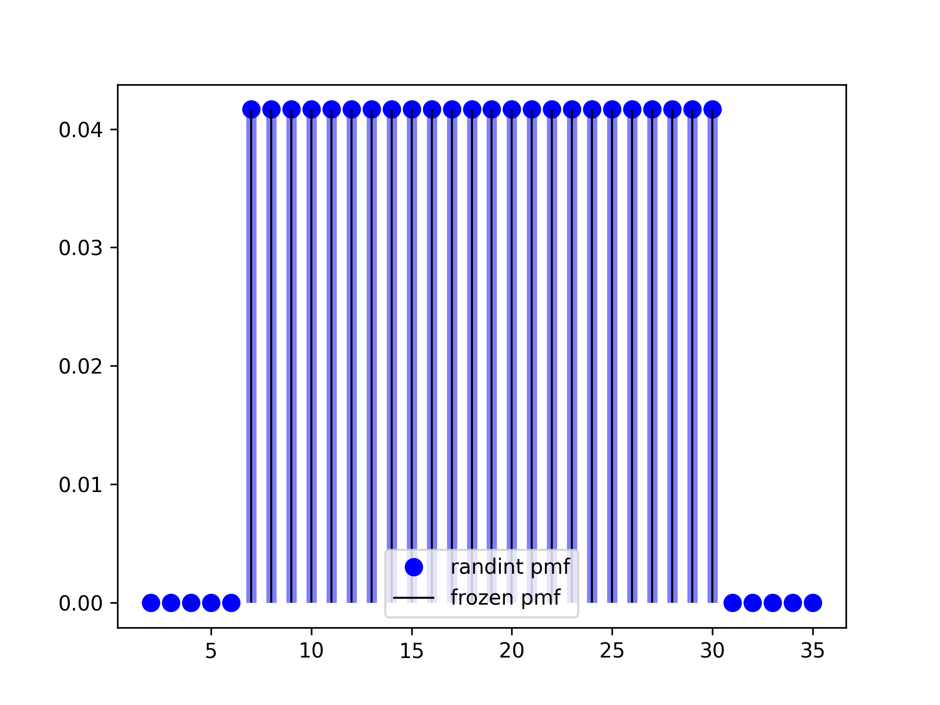
A uniform discrete random variable.

Extended Summary

%(before_notes)s

Notes

The probability mass function for randint is:

f (k) = \frac{1}{high - low}

for $k \in {low, \dots, high - 1}$ .

randint takes $low$ and $high$ as shape parameters.

%(after_notes)s

Examples

import numpy as np
from scipy.stats import randint
import matplotlib.pyplot as plt
fig, ax = plt.subplots(1, 1)

✓

Calculate the first four moments:

low, high = 7, 31
mean, var, skew, kurt = randint.stats(low, high, moments='mvsk')

✓

Display the probability mass function (``pmf``):

x = np.arange(low - 5, high + 5)

✓

ax.plot(x, randint.pmf(x, low, high), 'bo', ms=8, label='randint pmf')
ax.vlines(x, 0, randint.pmf(x, low, high), colors='b', lw=5, alpha=0.5)

✗

Alternatively, the distribution object can be called (as a function) to fix the shape and location. This returns a "frozen" RV object holding the given parameters fixed. Freeze the distribution and display the frozen ``pmf``:

rv = randint(low, high)

✓

ax.vlines(x, 0, rv.pmf(x), colors='k', linestyles='-',
          lw=1, label='frozen pmf')
ax.legend(loc='lower center')

✗

plt.show()

✓

Check the relationship between the cumulative distribution function (``cdf``) and its inverse, the percent point function (``ppf``):

q = np.arange(low, high)
p = randint.cdf(q, low, high)
np.allclose(q, randint.ppf(p, low, high))

✓

Generate random numbers:

r = randint.rvs(low, high, size=1000)

✓

Aliases

scipy.stats._discrete_distns.randint_gen