{ } Raw JSON

bundles / scipy 1.17.1 / scipy / stats / _kde / gaussian_kde

class

`scipy.stats._kde:gaussian_kde`

source: /scipy/stats/_kde.py :36

Signature

class gaussian_kde ( dataset , bw_method = None , weights = None )

Members

Summary

Representation of a kernel-density estimate using Gaussian kernels.

Extended Summary

Kernel density estimation is a way to estimate the probability density function (PDF) of a random variable in a non-parametric way. gaussian_kde works for both uni-variate and multi-variate data. It includes automatic bandwidth determination. The estimation works best for a unimodal distribution; bimodal or multi-modal distributions tend to be oversmoothed.

Parameters

dataset : array_like: Datapoints to estimate from. In case of univariate data this is a 1-D array, otherwise a 2-D array with shape (# of dims, # of data).
bw_method : str, scalar or callable, optional: The method used to calculate the bandwidth factor. This can be 'scott', 'silverman', a scalar constant or a callable. If a scalar, this will be used directly as factor. If a callable, it should take a gaussian_kde instance as only parameter and return a scalar. If None (default), 'scott' is used. See Notes for more details.
weights : array_like, optional: weights of datapoints. This must be the same shape as dataset. If None (default), the samples are assumed to be equally weighted

Attributes

dataset : ndarray: The dataset with which gaussian_kde was initialized.
d : int: Number of dimensions.
n : int: Number of datapoints.
neff : int: Effective number of datapoints.
versionadded 1.2.0
factor : float: The bandwidth factor obtained from covariance_factor.
covariance : ndarray: The kernel covariance matrix; this is the data covariance matrix multiplied by the square of the bandwidth factor, e.g. np.cov(dataset) * factor**2.
inv_cov : ndarray: The inverse of covariance.

Methods

evaluate
__call__
integrate_gaussian
integrate_box_1d
integrate_box
integrate_kde
pdf
logpdf
resample
set_bandwidth
covariance_factor
marginal

Notes

Bandwidth selection strongly influences the estimate obtained from the KDE (much more so than the actual shape of the kernel). Bandwidth selection can be done by a "rule of thumb", by cross-validation, by "plug-in methods" or by other means; see ^[3], ^[4] for reviews. gaussian_kde uses a rule of thumb, the default is Scott's Rule.

Scott's Rule ^[1], implemented as scotts_factor, is

n**(-1./(d+4)),

with n the number of data points and d the number of dimensions. In the case of unequally weighted points, scotts_factor becomes

neff**(-1./(d+4)),

with neff the effective number of datapoints. Silverman's suggestion for multivariate data ^[2], implemented as silverman_factor, is

(n * (d + 2) / 4.)**(-1. / (d + 4)).

or in the case of unequally weighted points

(neff * (d + 2) / 4.)**(-1. / (d + 4)).

Note that this is not the same as "Silverman's rule of thumb" ^[6], which may be more robust in the univariate case; see documentation of the set_bandwidth method for implementing a custom bandwidth rule.

Good general descriptions of kernel density estimation can be found in ^[1] and ^[2], the mathematics for this multi-dimensional implementation can be found in ^[1].

With a set of weighted samples, the effective number of datapoints neff is defined by

neff = sum(weights)^2 / sum(weights^2)

as detailed in ^[5].

gaussian_kde does not currently support data that lies in a lower-dimensional subspace of the space in which it is expressed. For such data, consider performing principal component analysis / dimensionality reduction and using gaussian_kde with the transformed data.

Examples

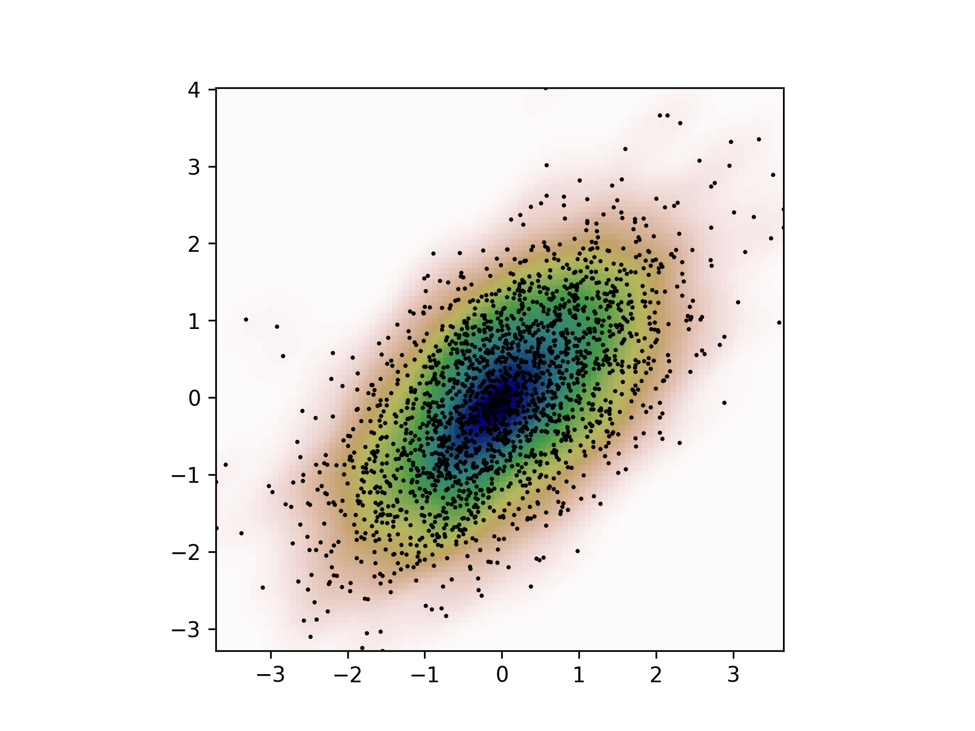
Generate some random two-dimensional data:

import numpy as np
from scipy import stats
def measure(n):
    "Measurement model, return two coupled measurements."
    m1 = np.random.normal(size=n)
    m2 = np.random.normal(scale=0.5, size=n)
    return m1+m2, m1-m2

✓

m1, m2 = measure(2000)
xmin = m1.min()
xmax = m1.max()
ymin = m2.min()
ymax = m2.max()

✓

Perform a kernel density estimate on the data:

X, Y = np.mgrid[xmin:xmax:100j, ymin:ymax:100j]
positions = np.vstack([X.ravel(), Y.ravel()])
values = np.vstack([m1, m2])
kernel = stats.gaussian_kde(values)
Z = np.reshape(kernel(positions).T, X.shape)

✓

Plot the results:

import matplotlib.pyplot as plt
fig, ax = plt.subplots()

✓

ax.imshow(np.rot90(Z), cmap=plt.cm.gist_earth_r,
          extent=[xmin, xmax, ymin, ymax])
ax.plot(m1, m2, 'k.', markersize=2)
ax.set_xlim([xmin, xmax])
ax.set_ylim([ymin, ymax])

✗

plt.show()

✓

Compare against manual KDE at a point:

point = [1, 2]
mean = values.T
cov = kernel.factor**2 * np.cov(values)
X = stats.multivariate_normal(cov=cov)
res = kernel.pdf(point)
ref = X.pdf(point - mean).sum() / len(mean)
np.allclose(res, ref)