bundles / scipy 2.0.0.dev0+git20260907.41eeb59 / scipy / integrate / _ivp / rk / RK23

class

`scipy.integrate._ivp.rk:RK23`

source: build-install/usr/lib/python3.14/site-packages/scipy/integrate/_ivp/rk.py:183

Signature

class RK23(fun, t0, y0, t_bound, max_step = inf, rtol = 0.001, atol = 1e-06, vectorized = False, first_step = None, **extraneous)

Summary

Explicit Runge-Kutta method of order 3(2).

Extended Summary

This uses the Bogacki-Shampine pair of formulas ^[1]. The error is controlled assuming accuracy of the second-order method, but steps are taken using the third-order accurate formula (local extrapolation is done). A cubic Hermite polynomial is used for the dense output.

Can be applied in the complex domain.

Parameters

fun : callable

Right-hand side of the system: the time derivative of the state y at time t. The calling signature is fun(t, y), where t is a scalar and y is an ndarray with len(y) = len(y0). fun must return an array of the same shape as y. See vectorized for more information.

t0 : float

Initial time.

y0 : array_like, shape (n,)

Initial state.

t_bound : float

Boundary time - the integration won't continue beyond it. It also determines the direction of the integration.

max_step : float, optional

Maximum allowed step size. Default is np.inf, i.e., the step size is not bounded and determined solely by the solver.

rtol, atol : float and array_like, optional

Relative and absolute tolerances. The solver keeps the local error estimates less than atol + rtol * abs(y). Here rtol controls a relative accuracy (number of correct digits), while atol controls absolute accuracy (number of correct decimal places). To achieve the desired rtol, set atol to be smaller than the smallest value that can be expected from rtol * abs(y) so that rtol dominates the allowable error. If atol is larger than rtol * abs(y) the number of correct digits is not guaranteed. Conversely, to achieve the desired atol set rtol such that rtol * abs(y) is always smaller than atol. If components of y have different scales, it might be beneficial to set different atol values for different components by passing array_like with shape (n,) for atol. Default values are 1e-3 for rtol and 1e-6 for atol.

vectorized : bool, optional

Whether fun may be called in a vectorized fashion. False (default) is recommended for this solver.

If vectorized is False, fun will always be called with y of shape (n,), where n = len(y0).

If vectorized is True, fun may be called with y of shape (n, k), where k is an integer. In this case, fun must behave such that fun(t, y)[:, i] == fun(t, y[:, i]) (i.e. each column of the returned array is the time derivative of the state corresponding with a column of y).

Setting vectorized=True allows for faster finite difference approximation of the Jacobian by methods 'Radau' and 'BDF', but will result in slower execution for this solver.

first_step : float or None, optional

Initial step size. Default is None which means that the algorithm should choose.

**extraneous

Any additional keyword arguments will be ignored.

Attributes

n : int: Number of equations.
status : str: Current status of the solver: 'running', 'finished' or 'failed'.
t_bound : float: Boundary time.
direction : float: Integration direction: +1 or -1.
t : float: Current time.
y : ndarray: Current state.
t_old : float: Previous time. None if no steps were made yet.
step_size : float: Size of the last successful step. None if no steps were made yet.
nfev : int: Number evaluations of the system's right-hand side.
njev : int: Number of evaluations of the Jacobian. Is always 0 for this solver as it does not use the Jacobian.
nlu : int: Number of LU decompositions. Is always 0 for this solver.

Examples

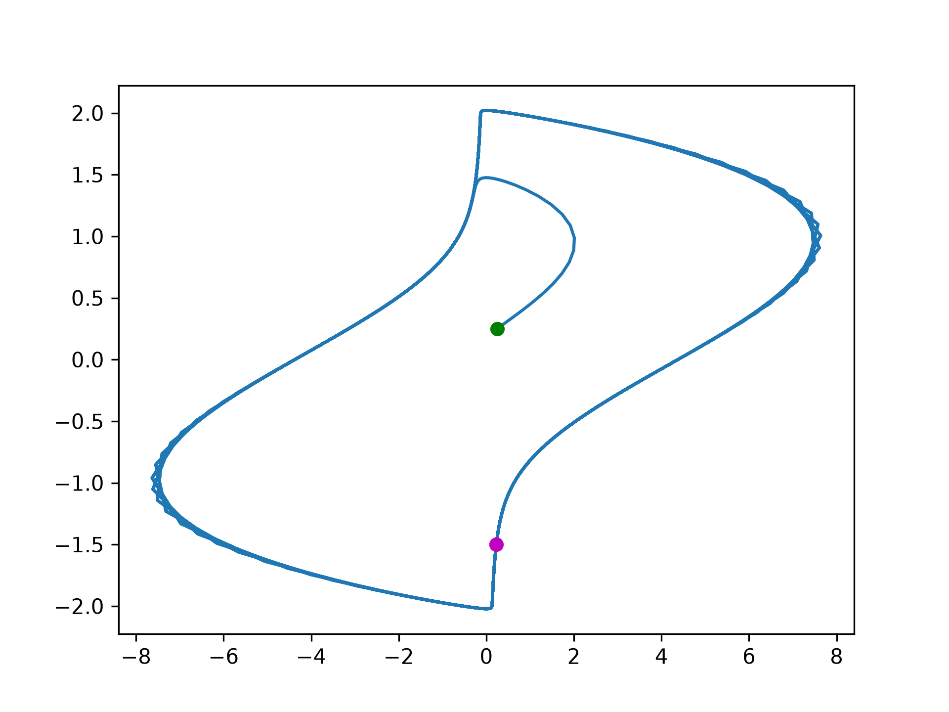
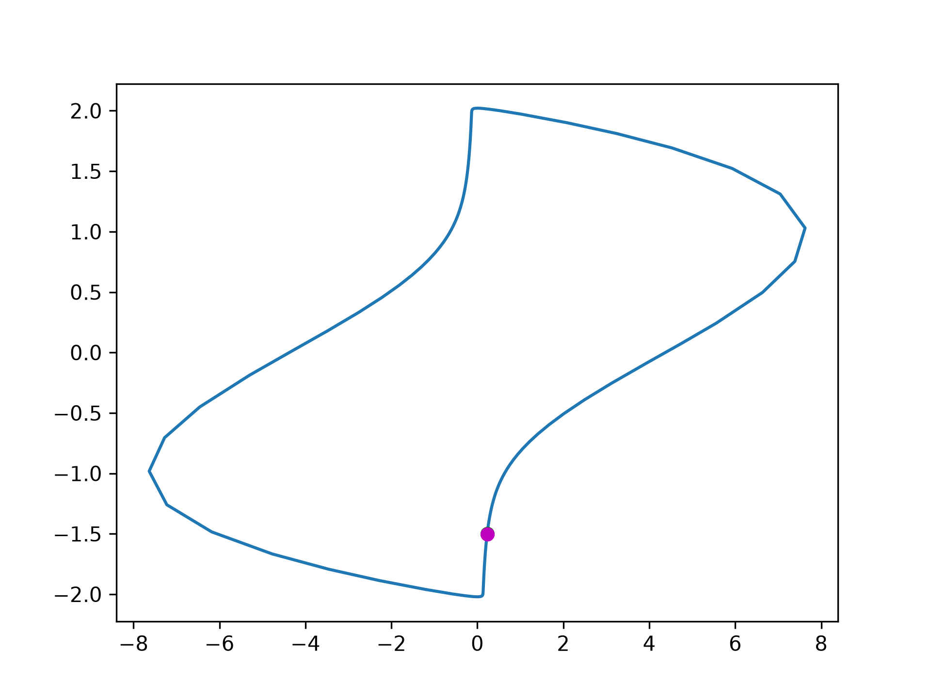
This example demonstrates how to compute one period of a periodic orbit in a two-dimensional dynamical system.

import numpy as np
import scipy.integrate as itg
import matplotlib.pylab as plt

✓

Define a function that returns the right-hand side of a dynamical system with a stable periodic orbit.

def dynam_sys(t, x):
    dx1_dt = 5*(1-x[1]**2)*x[0] - x[1]
    dx2_dt = x[0]
    return [dx1_dt, dx2_dt]

✓

The system has an equilibrium at the origin. Create a solver object with an initial state slightly away from the equilibrium.

solver = itg.RK45(dynam_sys, 0, [0.25,0.25], 1E200, max_step=0.05)

✓

Create an array in which to store the estimated solution. To allow for concatenation of future states, initialize the array by reshaping the initial state.

soly = solver.y.reshape(1, 2)

✓

To find a point on the periodic orbit, run the solver for ``2000`` integration steps. Store the estimated states in ``soly``.

for i in range(2000):
    solver.step()
    solyn = solver.y.reshape(1, 2)
    soly = np.concatenate((soly, solyn))

✓

Plot ``soly`` with its first element in green and its final element in magenta.

plt.plot(soly[:,0], soly[:,1])
plt.plot(soly[0,0], soly[0,1], "go")
plt.plot(soly[-1,0], soly[-1,1], "mo")

✗

[<matplotlib.lines.Line2D object at 0x7f3f687cae40>]

plt.show()

✓

The plot shows that the last element in ``soly`` is located on a segment of the periodic orbit where there is relatively little variation in the estimated states. Create another solver and initialize it with the last element in ``soly``.

init = np.array([soly[-1,0], soly[-1,1]])
POsolver = itg.RK23(dynam_sys, 0, init, 5000, max_step=0.05)

✓

Create a variable that tracks the distance of the current estimated state from the initial state. Run ``POsolver`` until the current estimated state is within ``0.005`` units of the last estimated state.

dist_init = 1
POsoly = POsolver.y.reshape(1, 2)
while dist_init > 0.005:
    POsolver.step()
    POsolyn = POsolver.y.reshape(1, 2)
    POsoly = np.concatenate((POsoly, POsolyn))
    dist_init = np.linalg.norm(init-POsolyn)

✓

Plot ``POsoly`` with its initial element in green and its final element in magenta.

plt.plot(POsoly[:,0], POsoly[:,1])
plt.plot(POsoly[0,0], POsoly[0,1], "go")
plt.plot(POsoly[-1,0], POsoly[-1,1], "mo")

✗

[<matplotlib.lines.Line2D object at 0x7f3f68ed3cb0>]

plt.show()

✓

The plot shows approximately one period of the orbit. The final and initial states are so close that the final state marker obscures the initial state marker.

Aliases

scipy.integrate.RK23