`scipy.special._orthogonal:jacobi`

source: build-install/usr/lib/python3.14/site-packages/scipy/special/_orthogonal.py:345

Signature

def jacobi(n, alpha, beta, monic = False)

Summary

Jacobi polynomial.

Extended Summary

Defined to be the solution of

(1 - x^{2}) \frac{d ^{2}}{d x ^{2}} P_{n}^{(α, β)} (x) + (β - α - (α + β + 2) x) \frac{d}{d x} P_{n}^{(α, β)} (x) + n (n + α + β + 1) P_{n}^{(α, β)} (x) = 0

for $α, β > - 1$ ; $P_{n}^{(α, β)}$ is a polynomial of degree $n$ .

Parameters

n : int: Degree of the polynomial.
alpha : float: Parameter, must be greater than -1.
beta : float: Parameter, must be greater than -1.
monic : bool, optional: If True, scale the leading coefficient to be 1. Default is False.

Returns

P : orthopoly1d: Jacobi polynomial.

Notes

For fixed $α, β$ , the polynomials $P_{n}^{(α, β)}$ are orthogonal over $[- 1, 1]$ with weight function $(1 - x)^{α} (1 + x)^{β}$ .

Examples

The Jacobi polynomials satisfy the recurrence relation: .. math:: P_n^{(\alpha, \beta-1)}(x) - P_n^{(\alpha-1, \beta)}(x) = P_{n-1}^{(\alpha, \beta)}(x) This can be verified, for example, for :math:`\alpha = \beta = 2` and :math:`n = 1` over the interval :math:`[-1, 1]`:

import numpy as np
from scipy.special import jacobi
x = np.arange(-1.0, 1.0, 0.01)
np.allclose(jacobi(0, 2, 2)(x),
            jacobi(1, 2, 1)(x) - jacobi(1, 1, 2)(x))

✓

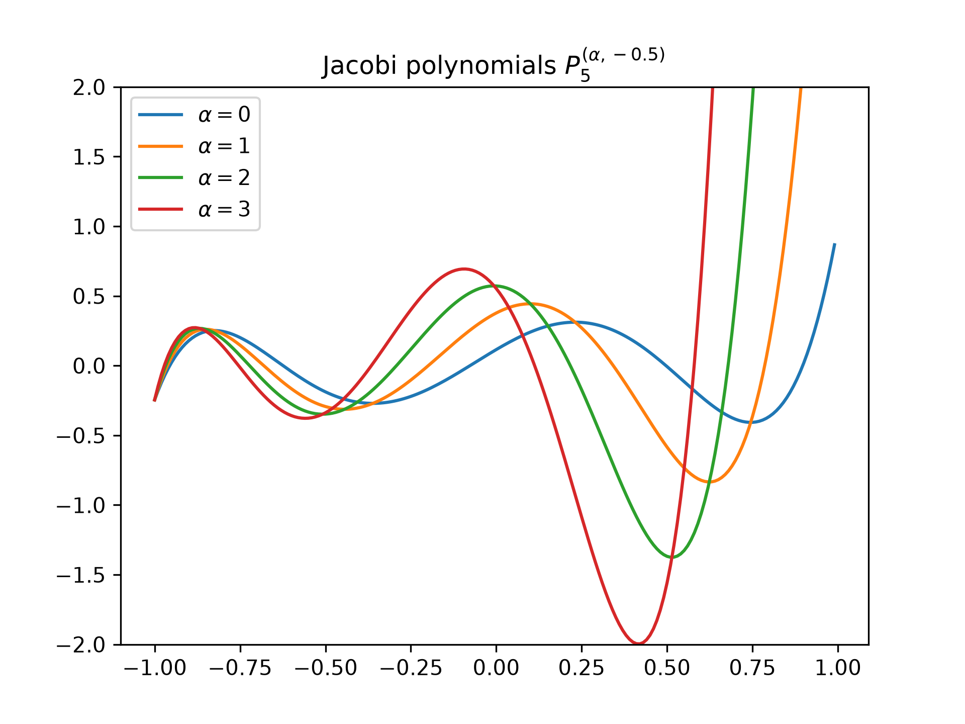
True

Plot of the Jacobi polynomial :math:`P_5^{(\alpha, -0.5)}` for different values of :math:`\alpha`:

import matplotlib.pyplot as plt
x = np.arange(-1.0, 1.0, 0.01)
fig, ax = plt.subplots()

✓

ax.set_ylim(-2.0, 2.0)
ax.set_title(r'Jacobi polynomials $P_5^{(\alpha, -0.5)}$')
for alpha in np.arange(0, 4, 1):
    ax.plot(x, jacobi(5, alpha, -0.5)(x), label=rf'$\alpha={alpha}$')
plt.legend(loc='best')

✗

<matplotlib.legend.Legend object at 0x7f3f601c3380>

plt.show()

✓