bundles / scipy 1.17.1 / scipy / integrate / _ivp / ivp / solve_ivp
function
scipy.integrate._ivp.ivp:solve_ivp
Signature
def solve_ivp ( fun , t_span , y0 , method = RK45 , t_eval = None , dense_output = False , events = None , vectorized = False , args = None , ** options ) Summary
Solve an initial value problem for a system of ODEs.
Extended Summary
This function numerically integrates a system of ordinary differential equations given an initial value
dy / dt = f(t, y)
y(t0) = y0
Here t is a 1-D independent variable (time), y(t) is an N-D vector-valued function (state), and an N-D vector-valued function f(t, y) determines the differential equations. The goal is to find y(t) approximately satisfying the differential equations, given an initial value y(t0)=y0.
Some of the solvers support integration in the complex domain, but note that for stiff ODE solvers, the right-hand side must be complex-differentiable (satisfy Cauchy-Riemann equations [11]). To solve a problem in the complex domain, pass y0 with a complex data type. Another option always available is to rewrite your problem for real and imaginary parts separately.
Parameters
fun: callableRight-hand side of the system: the time derivative of the state
yat timet. The calling signature isfun(t, y), wheretis a scalar andyis an ndarray withlen(y) = len(y0). Additional arguments need to be passed ifargsis used (see documentation ofargsargument).funmust return an array of the same shape asy. Seevectorizedfor more information.t_span: 2-member sequenceInterval of integration (t0, tf). The solver starts with t=t0 and integrates until it reaches t=tf. Both t0 and tf must be floats or values interpretable by the float conversion function.
y0: array_like, shape (n,)Initial state. For problems in the complex domain, pass
y0with a complex data type (even if the initial value is purely real).method: string or `OdeSolver`, optionalIntegration method to use:
'RK45' (default): Explicit Runge-Kutta method of order 5(4) [1]. The error is controlled assuming accuracy of the fourth-order method, but steps are taken using the fifth-order accurate formula (local extrapolation is done). A quartic interpolation polynomial is used for the dense output [2]. Can be applied in the complex domain.
'RK23': Explicit Runge-Kutta method of order 3(2) [3]. The error is controlled assuming accuracy of the second-order method, but steps are taken using the third-order accurate formula (local extrapolation is done). A cubic Hermite polynomial is used for the dense output. Can be applied in the complex domain.
'DOP853': Explicit Runge-Kutta method of order 8 [13]. Python implementation of the "DOP853" algorithm originally written in Fortran [14]. A 7-th order interpolation polynomial accurate to 7-th order is used for the dense output. Can be applied in the complex domain.
'Radau': Implicit Runge-Kutta method of the Radau IIA family of order 5 [4]. The error is controlled with a third-order accurate embedded formula. A cubic polynomial which satisfies the collocation conditions is used for the dense output.
'BDF': Implicit multi-step variable-order (1 to 5) method based on a backward differentiation formula for the derivative approximation [5]. The implementation follows the one described in [6]. A quasi-constant step scheme is used and accuracy is enhanced using the NDF modification. Can be applied in the complex domain.
'LSODA': Adams/BDF method with automatic stiffness detection and switching [7], [8]. This is a wrapper of the Fortran solver from ODEPACK.
Explicit Runge-Kutta methods ('RK23', 'RK45', 'DOP853') should be used for non-stiff problems and implicit methods ('Radau', 'BDF') for stiff problems [9]. Among Runge-Kutta methods, 'DOP853' is recommended for solving with high precision (low values of rtol and atol).
If not sure, first try to run 'RK45'. If it makes unusually many iterations, diverges, or fails, your problem is likely to be stiff and you should use 'Radau' or 'BDF'. 'LSODA' can also be a good universal choice, but it might be somewhat less convenient to work with as it wraps old Fortran code.
You can also pass an arbitrary class derived from OdeSolver which implements the solver.
t_eval: array_like or None, optionalTimes at which to store the computed solution, must be sorted and lie within
t_span. If None (default), use points selected by the solver.dense_output: bool, optionalWhether to compute a continuous solution. Default is False.
events: callable, or list of callables, optionalEvents to track. If None (default), no events will be tracked. Each event occurs at the zeros of a continuous function of time and state. Each function must have the signature
event(t, y)where additional argument have to be passed ifargsis used (see documentation ofargsargument). Each function must return a float. The solver will find an accurate value of t at whichevent(t, y(t)) = 0using a root-finding algorithm. By default, all zeros will be found. The solver looks for a sign change over each step, so if multiple zero crossings occur within one step, events may be missed. Additionally eacheventfunction might have the following attributes:terminal: bool or int, optional
When boolean, whether to terminate integration if this event occurs. When integral, termination occurs after the specified the number of occurrences of this event. Implicitly False if not assigned.
direction: float, optional
Direction of a zero crossing. If
directionis positive,eventwill only trigger when going from negative to positive, and vice versa ifdirectionis negative. If 0, then either direction will trigger event. Implicitly 0 if not assigned.
You can assign attributes like
event.terminal = Trueto any function in Python.vectorized: bool, optionalWhether
funcan be called in a vectorized fashion. Default is False.If
vectorizedis False,funwill always be called withyof shape(n,), wheren = len(y0).If
vectorizedis True,funmay be called withyof shape(n, k), wherekis an integer. In this case,funmust behave such thatfun(t, y)[:, i] == fun(t, y[:, i])(i.e. each column of the returned array is the time derivative of the state corresponding with a column ofy).Setting
vectorized=Trueallows for faster finite difference approximation of the Jacobian by methods 'Radau' and 'BDF', but will result in slower execution for other methods and for 'Radau' and 'BDF' in some circumstances (e.g. smalllen(y0)).args: tuple, optionalAdditional arguments to pass to the user-defined functions. If given, the additional arguments are passed to all user-defined functions. So if, for example,
funhas the signaturefun(t, y, a, b, c), then jac (if given) and any event functions must have the same signature, andargsmust be a tuple of length 3.**optionsOptions passed to a chosen solver. All options available for already implemented solvers are listed below.
first_step: float or None, optionalInitial step size. Default is
Nonewhich means that the algorithm should choose.max_step: float, optionalMaximum allowed step size. Default is np.inf, i.e., the step size is not bounded and determined solely by the solver.
rtol, atol: float or array_like, optionalRelative and absolute tolerances. The solver keeps the local error estimates less than
atol + rtol * abs(y). Here rtol controls a relative accuracy (number of correct digits), while atol controls absolute accuracy (number of correct decimal places). To achieve the desired rtol, set atol to be smaller than the smallest value that can be expected fromrtol * abs(y)so that rtol dominates the allowable error. If atol is larger thanrtol * abs(y)the number of correct digits is not guaranteed. Conversely, to achieve the desired atol set rtol such thatrtol * abs(y)is always smaller than atol. If components of y have different scales, it might be beneficial to set different atol values for different components by passing array_like with shape (n,) for atol. Default values are 1e-3 for rtol and 1e-6 for atol.jac: array_like, sparse_matrix, callable or None, optionalJacobian matrix of the right-hand side of the system with respect to y, required by the 'Radau', 'BDF' and 'LSODA' method. The Jacobian matrix has shape (n, n) and its element (i, j) is equal to
d f_i / d y_j. There are three ways to define the Jacobian:If array_like or sparse_matrix, the Jacobian is assumed to be constant. Not supported by 'LSODA'.
If callable, the Jacobian is assumed to depend on both t and y; it will be called as
jac(t, y), as necessary. Additional arguments have to be passed ifargsis used (see documentation ofargsargument). For 'Radau' and 'BDF' methods, the return value might be a sparse matrix.If None (default), the Jacobian will be approximated by finite differences.
It is generally recommended to provide the Jacobian rather than relying on a finite-difference approximation.
jac_sparsity: array_like, sparse matrix or None, optionalDefines a sparsity structure of the Jacobian matrix for a finite- difference approximation. Its shape must be (n, n). This argument is ignored if jac is not
None. If the Jacobian has only few non-zero elements in each row, providing the sparsity structure will greatly speed up the computations [10]. A zero entry means that a corresponding element in the Jacobian is always zero. If None (default), the Jacobian is assumed to be dense. Not supported by 'LSODA', see lband and uband instead.lband, uband: int or None, optionalParameters defining the bandwidth of the Jacobian for the 'LSODA' method, i.e.,
jac[i, j] != 0 only for i - lband <= j <= i + uband. Default is None. Setting these requires your jac routine to return the Jacobian in the packed format: the returned array must havencolumns anduband + lband + 1rows in which Jacobian diagonals are written. Specificallyjac_packed[uband + i - j , j] = jac[i, j]. The same format is used in scipy.linalg.solve_banded (check for an illustration). These parameters can be also used withjac=Noneto reduce the number of Jacobian elements estimated by finite differences.min_step: float, optionalThe minimum allowed step size for 'LSODA' method. By default min_step is zero.
Returns
: Bunch object with the following fields defined:t: ndarray, shape (n_points,)Time points.
y: ndarray, shape (n, n_points)Values of the solution at t.
sol: `OdeSolution` or NoneFound solution as OdeSolution instance; None if
dense_outputwas set to False.t_events: list of ndarray or NoneContains for each event type a list of arrays at which an event of that type event was detected. None if
eventswas None.y_events: list of ndarray or NoneFor each value of t_events, the corresponding value of the solution. None if
eventswas None.nfev: intNumber of evaluations of the right-hand side.
njev: intNumber of evaluations of the Jacobian.
nlu: intNumber of LU decompositions.
status: intReason for algorithm termination:
-1: Integration step failed.
0: The solver successfully reached the end of
tspan.1: A termination event occurred.
message: stringHuman-readable description of the termination reason.
success: boolTrue if the solver reached the interval end or a termination event occurred (
status >= 0).
Notes
Array API Standard Support
solve_ivp has experimental support for Python Array API Standard compatible backends in addition to NumPy. Please consider testing these features by setting an environment variable SCIPY_ARRAY_API=1 and providing CuPy, PyTorch, JAX, or Dask arrays as array arguments. The following combinations of backend and device (or other capability) are supported.
====================  ====================  ====================
Library               CPU                   GPU
====================  ====================  ====================
NumPy                 ✅                     n/a
CuPy                  n/a                   ⛔
PyTorch               ⛔                     ⛔
JAX                   ⛔                     ⛔
Dask                  ⛔                     n/a
====================  ====================  ====================
See
dev-arrayapifor more information.
Examples
Basic exponential decay showing automatically chosen time points.import numpy as np from scipy.integrate import solve_ivp def exponential_decay(t, y): return -0.5 * y sol = solve_ivp(exponential_decay, [0, 10], [2, 4, 8])✓
print(sol.t)
print(sol.y)
✗
sol = solve_ivp(exponential_decay, [0, 10], [2, 4, 8],
                t_eval=[0, 1, 2, 4, 10])
print(sol.t)
✓
print(sol.y)
✗def upward_cannon(t, y): return [y[1], -0.5] def hit_ground(t, y): return y[0] hit_ground.terminal = True hit_ground.direction = -1 sol = solve_ivp(upward_cannon, [0, 100], [0, 10], events=hit_ground) print(sol.t_events)✓
print(sol.t)
✗def apex(t, y): return y[1] sol = solve_ivp(upward_cannon, [0, 100], [0, 10], events=(hit_ground, apex), dense_output=True) print(sol.t_events)✓
print(sol.t)
print(sol.sol(sol.t_events[1][0]))
print(sol.y_events)
✗
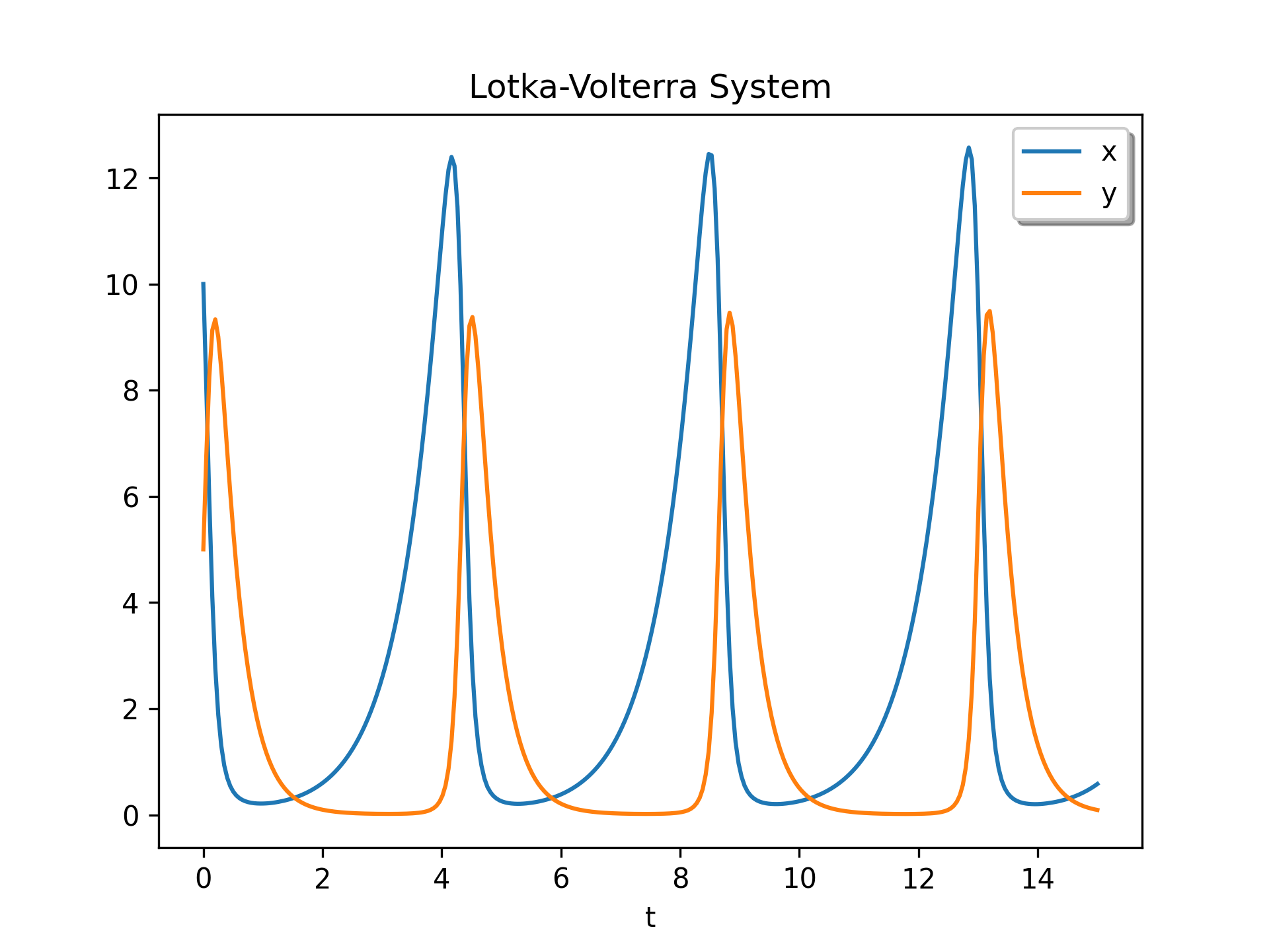
def lotkavolterra(t, z, a, b, c, d):
    x, y = z
    return [a*x - b*x*y, -c*y + d*x*y]
✓
sol = solve_ivp(lotkavolterra, [0, 15], [10, 5], args=(1.5, 1, 3, 1),
                dense_output=True)
✓
t = np.linspace(0, 15, 300)
z = sol.sol(t)
import matplotlib.pyplot as plt
✓
plt.plot(t, z.T)
plt.xlabel('t')
plt.legend(['x', 'y'], shadow=True)
plt.title('Lotka-Volterra System')
✗
plt.show()
✓
A = np.array([[-0.25 + 0.14j, 0, 0.33 + 0.44j],
              [0.25 + 0.58j, -0.2 + 0.14j, 0],
              [0, 0.2 + 0.4j, -0.1 + 0.97j]])
✓
def deriv_vec(t, y):
    return A @ y
result = solve_ivp(deriv_vec, [0, 25],
                   np.array([10 + 0j, 20 + 0j, 30 + 0j]),
                   t_eval=np.linspace(0, 25, 101))
print(result.y[:, 0])
✓
print(result.y[:, -1])
✗def deriv_mat(t, y): return (A @ y.reshape(3, 3)).flatten() y0 = np.array([[2 + 0j, 3 + 0j, 4 + 0j], [5 + 0j, 6 + 0j, 7 + 0j], [9 + 0j, 34 + 0j, 78 + 0j]])✓
result = solve_ivp(deriv_mat, [0, 25], y0.flatten(),
                   t_eval=np.linspace(0, 25, 101))
print(result.y[:, 0].reshape(3, 3))
✓
print(result.y[:, -1].reshape(3, 3))
✗Aliases
-
scipy.integrate.solve_ivp