bundles / scipy 1.17.1 / scipy / integrate / _odepack_py / odeint

function

`scipy.integrate._odepack_py:odeint`

source: /scipy/integrate/_odepack_py.py :31

Signature

   def     odeint (    func    ,    y0    ,    t    ,    args    =  ()   ,    Dfun    =  None   ,    col_deriv    =  0   ,    full_output    =  0   ,    ml    =  None   ,    mu    =  None   ,    rtol    =  None   ,    atol    =  None   ,    tcrit    =  None   ,    h0    =  0.0   ,    hmax    =  0.0   ,    hmin    =  0.0   ,    ixpr    =  0   ,    mxstep    =  0   ,    mxhnil    =  0   ,    mxordn    =  12   ,    mxords    =  5   ,    printmessg    =  0   ,    tfirst    =  False     )

Summary

Integrate a system of ordinary differential equations.

Extended Summary

Solve a system of ordinary differential equations using lsoda from the FORTRAN library odepack.

Solves the initial value problem for stiff or non-stiff systems of first order ode-s

dy/dt = func(y, t, ...)  [or func(t, y, ...)]

where y can be a vector.

Parameters

func : callable(y, t, ...) or callable(t, y, ...): Computes the derivative of y at t. If the signature is callable(t, y, ...), then the argument tfirst must be set True. func must not modify the data in y, as it is a view of the data used internally by the ODE solver.
y0 : array: Initial condition on y (can be a vector).
t : array: A sequence of time points for which to solve for y. The initial value point should be the first element of this sequence. This sequence must be monotonically increasing or monotonically decreasing; repeated values are allowed.
args : tuple, optional: Extra arguments to pass to function.
Dfun : callable(y, t, ...) or callable(t, y, ...): Gradient (Jacobian) of func. If the signature is callable(t, y, ...), then the argument tfirst must be set True. Dfun must not modify the data in y, as it is a view of the data used internally by the ODE solver.
col_deriv : bool, optional: True if Dfun defines derivatives down columns (faster), otherwise Dfun should define derivatives across rows.
full_output : bool, optional: True if to return a dictionary of optional outputs as the second output
printmessg : bool, optional: Whether to print the convergence message
tfirst : bool, optional: If True, the first two arguments of func (and Dfun, if given) must t, y instead of the default y, t.
versionadded 1.1.0

Returns

y : array, shape (len(t), len(y0))

Array containing the value of y for each desired time in t, with the initial value y0 in the first row.

infodict : dict, only returned if full_output == True

Dictionary containing additional output information

=======  ============================================================
key      meaning
=======  ============================================================
'hu'     vector of step sizes successfully used for each time step
'tcur'   vector with the value of t reached for each time step
         (will always be at least as large as the input times)
'tolsf'  vector of tolerance scale factors, greater than 1.0,
         computed when a request for too much accuracy was detected
'tsw'    value of t at the time of the last method switch
         (given for each time step)
'nst'    cumulative number of time steps
'nfe'    cumulative number of function evaluations for each time step
'nje'    cumulative number of jacobian evaluations for each time step
'nqu'    a vector of method orders for each successful step
'imxer'  index of the component of largest magnitude in the
         weighted local error vector (e / ewt) on an error return, -1
         otherwise
'lenrw'  the length of the double work array required
'leniw'  the length of integer work array required
'mused'  a vector of method indicators for each successful time step:
         1: adams (nonstiff), 2: bdf (stiff)
=======  ============================================================

Other Parameters

ml, mu : int, optional: If either of these are not None or non-negative, then the Jacobian is assumed to be banded. These give the number of lower and upper non-zero diagonals in this banded matrix. For the banded case, Dfun should return a matrix whose rows contain the non-zero bands (starting with the lowest diagonal). Thus, the return matrix jac from Dfun should have shape (ml + mu + 1, len(y0)) when ml >=0 or mu >=0. The data in jac must be stored such that jac[i - j + mu, j] holds the derivative of the ith equation with respect to the jth state variable. If col_deriv is True, the transpose of this jac must be returned.
rtol, atol : float, optional: The input parameters rtol and atol determine the error control performed by the solver. The solver will control the vector, e, of estimated local errors in y, according to an inequality of the form max-norm of (e / ewt) <= 1, where ewt is a vector of positive error weights computed as ewt = rtol * abs(y) + atol. rtol and atol can be either vectors the same length as y or scalars. Defaults to 1.49012e-8.
tcrit : ndarray, optional: Vector of critical points (e.g., singularities) where integration care should be taken.
h0 : float, (0: solver-determined), optional: The step size to be attempted on the first step.
hmax : float, (0: solver-determined), optional: The maximum absolute step size allowed.
hmin : float, (0: solver-determined), optional: The minimum absolute step size allowed.
ixpr : bool, optional: Whether to generate extra printing at method switches.
mxstep : int, (0: solver-determined), optional: Maximum number of (internally defined) steps allowed for each integration point in t.
mxhnil : int, (0: solver-determined), optional: Maximum number of messages printed.
mxordn : int, (0: solver-determined), optional: Maximum order to be allowed for the non-stiff (Adams) method.
mxords : int, (0: solver-determined), optional: Maximum order to be allowed for the stiff (BDF) method.

Notes

Array API Standard Support

odeint is not in-scope for support of Python Array API Standard compatible backends other than NumPy.

See dev-arrayapi for more information.

Examples

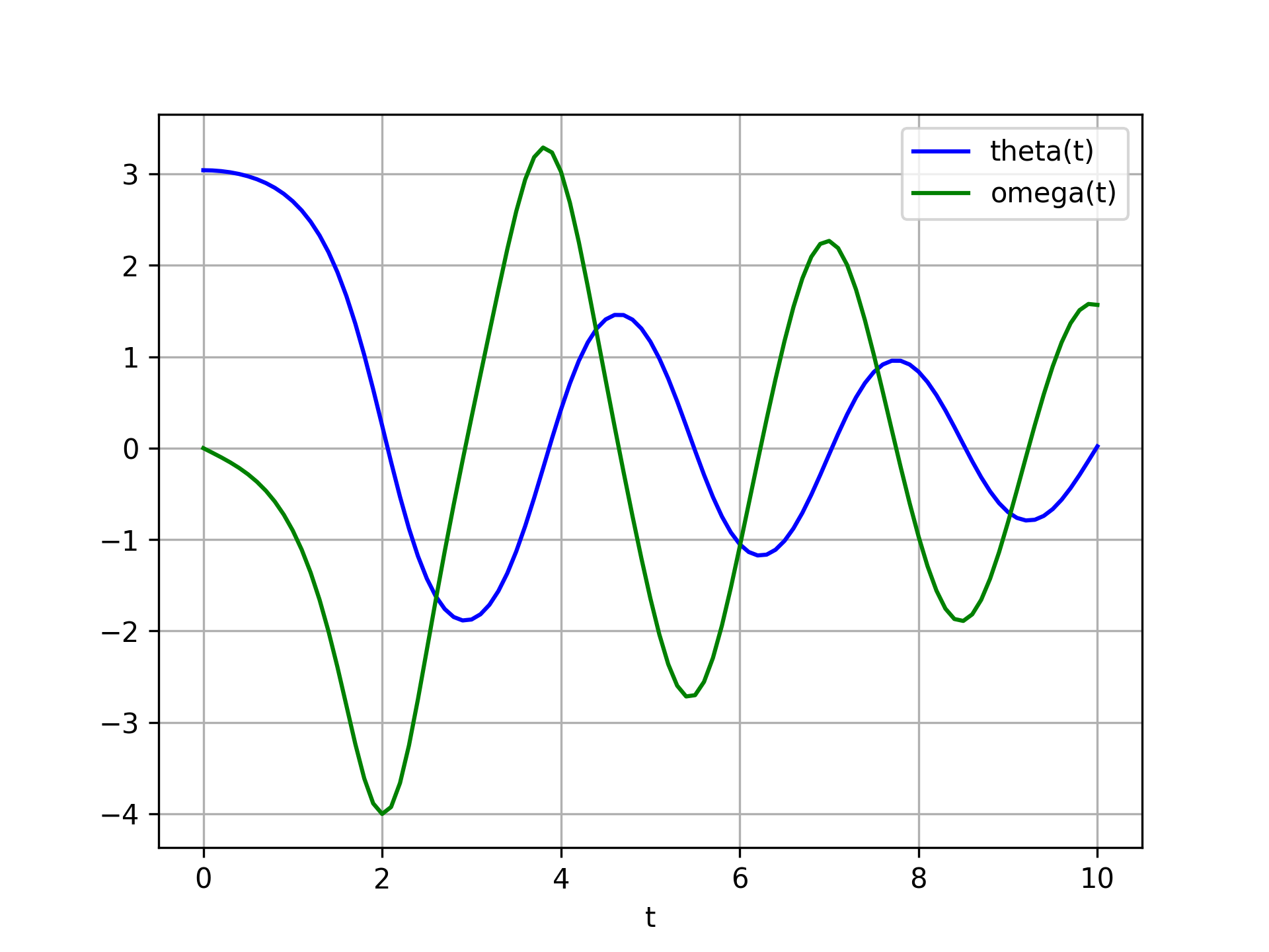
The second order differential equation for the angle `theta` of a pendulum acted on by gravity with friction can be written:: theta''(t) + b*theta'(t) + c*sin(theta(t)) = 0 where `b` and `c` are positive constants, and a prime (') denotes a derivative. To solve this equation with `odeint`, we must first convert it to a system of first order equations. By defining the angular velocity ``omega(t) = theta'(t)``, we obtain the system:: theta'(t) = omega(t) omega'(t) = -b*omega(t) - c*sin(theta(t)) Let `y` be the vector [`theta`, `omega`]. We implement this system in Python as:

import numpy as np
def pend(y, t, b, c):
    theta, omega = y
    dydt = [omega, -b*omega - c*np.sin(theta)]
    return dydt

✓

We assume the constants are `b` = 0.25 and `c` = 5.0:

b = 0.25
c = 5.0

✓

For initial conditions, we assume the pendulum is nearly vertical with `theta(0)` = `pi` - 0.1, and is initially at rest, so `omega(0)` = 0. Then the vector of initial conditions is

y0 = [np.pi - 0.1, 0.0]

✓

We will generate a solution at 101 evenly spaced samples in the interval 0 <= `t` <= 10. So our array of times is:

t = np.linspace(0, 10, 101)

✓

Call `odeint` to generate the solution. To pass the parameters `b` and `c` to `pend`, we give them to `odeint` using the `args` argument.

from scipy.integrate import odeint
sol = odeint(pend, y0, t, args=(b, c))

✓

The solution is an array with shape (101, 2). The first column is `theta(t)`, and the second is `omega(t)`. The following code plots both components.

import matplotlib.pyplot as plt

✓

plt.plot(t, sol[:, 0], 'b', label='theta(t)')
plt.plot(t, sol[:, 1], 'g', label='omega(t)')
plt.legend(loc='best')
plt.xlabel('t')

✗

plt.grid()
plt.show()

✓

Aliases

scipy.integrate.odeint

`scipy.integrate._odepack_py:odeint`

Signature

Summary

Extended Summary

Parameters

Returns

Other Parameters

Notes

Examples

See also

Aliases

Referenced by

This package