bundles / scipy 1.17.1 / scipy / interpolate / _bary_rational / AAA

class

`scipy.interpolate._bary_rational:AAA`

source: /scipy/interpolate/_bary_rational.py :213

Signature

   class     AAA (    x    ,    y    ,  * ,     rtol    =  None   ,    max_terms    =  100   ,    clean_up    =  True   ,    clean_up_tol    =  1e-13     )

Members

Summary

AAA real or complex rational approximation.

Extended Summary

As described in ^[1], the AAA algorithm is a greedy algorithm for approximation by rational functions on a real or complex set of points. The rational approximation is represented in a barycentric form from which the roots (zeros), poles, and residues can be computed.

Parameters

x : 1D array_like, shape (n,): 1-D array containing values of the independent variable. Values may be real or complex but must be finite.
y : 1D array_like, shape (n,): Function values f(x). Infinite and NaN values of values and corresponding values of points will be discarded.
rtol : float, optional: Relative tolerance, defaults to eps**0.75. If a small subset of the entries in values are much larger than the rest the default tolerance may be too loose. If the tolerance is too tight then the approximation may contain Froissart doublets or the algorithm may fail to converge entirely.
max_terms : int, optional: Maximum number of terms in the barycentric representation, defaults to 100. Must be greater than or equal to one.
clean_up : bool, optional: Automatic removal of Froissart doublets, defaults to True. See notes for more details.
clean_up_tol : float, optional: Poles with residues less than this number times the geometric mean of values times the minimum distance to points are deemed spurious by the cleanup procedure, defaults to 1e-13. See notes for more details.

Attributes

support_points : array: Support points of the approximation. These are a subset of the provided x at which the approximation strictly interpolates y. See notes for more details.
support_values : array: Value of the approximation at the support_points.
weights : array: Weights of the barycentric approximation.
errors : array: Error $∣ f (z) - r (z) ∣_{\infty}$ over points in the successive iterations of AAA.

Warns

: RuntimeWarning: If rtol is not achieved in max_terms iterations.

Notes

At iteration $m$ (at which point there are $m$ terms in the both the numerator and denominator of the approximation), the rational approximation in the AAA algorithm takes the barycentric form

r (z) = n (z) / d (z) = \frac{\sum _{j = 1}^{m} w _{j} f _{j} / ( z - z _{j} )}{\sum _{j = 1}^{m} w _{j} / ( z - z _{j} )},

where $z_{1}, \dots, z_{m}$ are real or complex support points selected from x, $f_{1}, \dots, f_{m}$ are the corresponding real or complex data values from y, and $w_{1}, \dots, w_{m}$ are real or complex weights.

Each iteration of the algorithm has two parts: the greedy selection the next support point and the computation of the weights. The first part of each iteration is to select the next support point to be added $z_{m + 1}$ from the remaining unselected x, such that the nonlinear residual $∣ f (z_{m + 1}) - n (z_{m + 1}) / d (z_{m + 1}) ∣$ is maximised. The algorithm terminates when this maximum is less than rtol * np.linalg.norm(f, ord=np.inf). This means the interpolation property is only satisfied up to a tolerance, except at the support points where approximation exactly interpolates the supplied data.

In the second part of each iteration, the weights $w_{j}$ are selected to solve the least-squares problem

minimise_{w_{j}} ∣ f d - n ∣ subject to j = 1 \sum m + 1 w_{j} = 1,

over the unselected elements of x.

One of the challenges with working with rational approximations is the presence of Froissart doublets, which are either poles with vanishingly small residues or pole-zero pairs that are close enough together to nearly cancel, see ^[2]. The greedy nature of the AAA algorithm means Froissart doublets are rare. However, if rtol is set too tight then the approximation will stagnate and many Froissart doublets will appear. Froissart doublets can usually be removed by removing support points and then resolving the least squares problem. The support point $z_{j}$ , which is the closest support point to the pole $a$ with residue $α$ , is removed if the following is satisfied

∣ α ∣/∣ z_{j} - a ∣ < clean_up_tol \cdot \tilde{f},

where $\tilde{f}$ is the geometric mean of support_values.

Examples

Here we reproduce a number of the numerical examples from [1]_ as a demonstration of the functionality offered by this method.

import numpy as np
import matplotlib.pyplot as plt
from scipy.interpolate import AAA
import warnings

✓

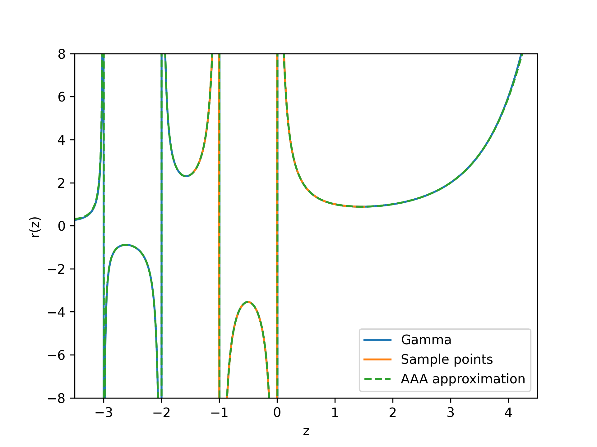
For the first example we approximate the gamma function on ``[-3.5, 4.5]`` by extrapolating from 100 samples in ``[-1.5, 1.5]``.

from scipy.special import gamma
sample_points = np.linspace(-1.5, 1.5, num=100)
r = AAA(sample_points, gamma(sample_points))
z = np.linspace(-3.5, 4.5, num=1000)
fig, ax = plt.subplots()

✓

ax.plot(z, gamma(z), label="Gamma")
ax.plot(sample_points, gamma(sample_points), label="Sample points")
ax.plot(z, r(z).real, '--', label="AAA approximation")
ax.set(xlabel="z", ylabel="r(z)", ylim=[-8, 8], xlim=[-3.5, 4.5])
ax.legend()

✗

plt.show()

✓

We can also view the poles of the rational approximation and their residues:

order = np.argsort(r.poles())

✓

r.poles()[order]
r.residues()[order]

✗

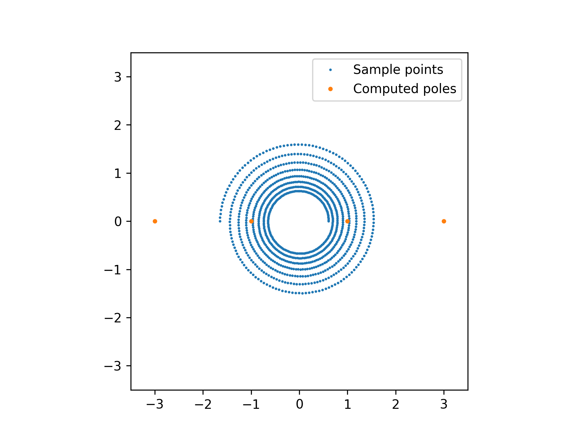
For the second example, we call `AAA` with a spiral of 1000 points that wind 7.5 times around the origin in the complex plane.

z = np.exp(np.linspace(-0.5, 0.5 + 15j*np.pi, 1000))
r = AAA(z, np.tan(np.pi*z/2), rtol=1e-13)

✓

We see that AAA takes 12 steps to converge with the following errors:

r.errors.size

✓

r.errors

✗

We can also plot the computed poles:

fig, ax = plt.subplots()

✓

ax.plot(z.real, z.imag, '.', markersize=2, label="Sample points")
ax.plot(r.poles().real, r.poles().imag, '.', markersize=5,
        label="Computed poles")
ax.set(xlim=[-3.5, 3.5], ylim=[-3.5, 3.5], aspect="equal")
ax.legend()

✗

plt.show()

✓

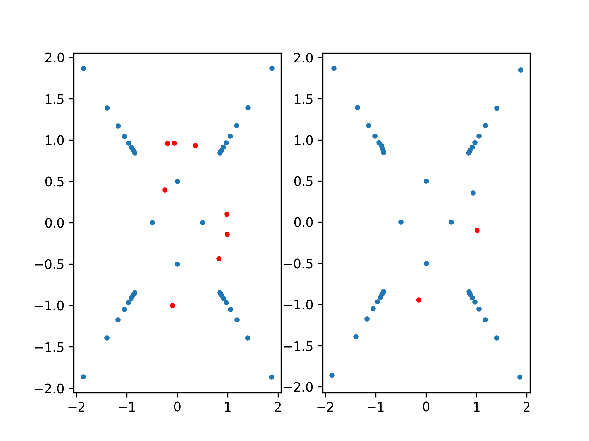
We now demonstrate the removal of Froissart doublets using the `clean_up` method using an example from [1]_. Here we approximate the function :math:`f(z)=\log(2 + z^4)/(1 + 16z^4)` by sampling it at 1000 roots of unity. The algorithm is run with ``rtol=0`` and ``clean_up=False`` to deliberately cause Froissart doublets to appear.

z = np.exp(1j*2*np.pi*np.linspace(0,1, num=1000))
def f(z):
    return np.log(2 + z**4)/(1 - 16*z**4)
with warnings.catch_warnings():  # filter convergence warning due to rtol=0
    warnings.simplefilter('ignore', RuntimeWarning)
    r = AAA(z, f(z), rtol=0, max_terms=50, clean_up=False)
mask = np.abs(r.residues()) < 1e-13
fig, axs = plt.subplots(ncols=2)

✓

axs[0].plot(r.poles().real[~mask], r.poles().imag[~mask], '.')
axs[0].plot(r.poles().real[mask], r.poles().imag[mask], 'r.')

✗

Now we call the `clean_up` method to remove Froissart doublets.

with warnings.catch_warnings():
    warnings.simplefilter('ignore', RuntimeWarning)
    r.clean_up()

✗

mask = np.abs(r.residues()) < 1e-13

✓

axs[1].plot(r.poles().real[~mask], r.poles().imag[~mask], '.')
axs[1].plot(r.poles().real[mask], r.poles().imag[mask], 'r.')

✗

plt.show()

✓

The left image shows the poles prior of the approximation ``clean_up=False`` with poles with residue less than ``10^-13`` in absolute value shown in red. The right image then shows the poles after the `clean_up` method has been called.

Aliases

scipy.interpolate.AAA