`scipy.interpolate._polyint:approximate_taylor_polynomial`

source: /scipy/interpolate/_polyint.py :462

Signature

   def     approximate_taylor_polynomial (    f    ,    x    ,    degree    ,    scale    ,    order    =  None     )

Summary

Estimate the Taylor polynomial of f at x by polynomial fitting.

Parameters

f : callable: The function whose Taylor polynomial is sought. Should accept a vector of x values.
x : scalar: The point at which the polynomial is to be evaluated.
degree : int: The degree of the Taylor polynomial
scale : scalar: The width of the interval to use to evaluate the Taylor polynomial. Function values spread over a range this wide are used to fit the polynomial. Must be chosen carefully.
order : int or None, optional: The order of the polynomial to be used in the fitting; f will be evaluated order+1 times. If None, use degree.

Returns

p : poly1d instance: The Taylor polynomial (translated to the origin, so that for example p(0)=f(x)).

Notes

The appropriate choice of "scale" is a trade-off; too large and the function differs from its Taylor polynomial too much to get a good answer, too small and round-off errors overwhelm the higher-order terms. The algorithm used becomes numerically unstable around order 30 even under ideal circumstances.

Choosing order somewhat larger than degree may improve the higher-order terms.

Examples

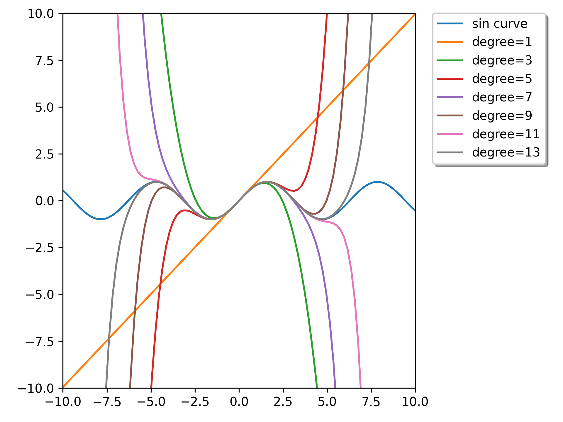
We can calculate Taylor approximation polynomials of sin function with various degrees:

import numpy as np
import matplotlib.pyplot as plt
from scipy.interpolate import approximate_taylor_polynomial
x = np.linspace(-10.0, 10.0, num=100)

✓

plt.plot(x, np.sin(x), label="sin curve")
for degree in np.arange(1, 15, step=2):
    sin_taylor = approximate_taylor_polynomial(np.sin, 0, degree, 1,
                                               order=degree + 2)
    plt.plot(x, sin_taylor(x), label=f"degree={degree}")
plt.legend(bbox_to_anchor=(1.05, 1), loc='upper left',
           borderaxespad=0.0, shadow=True)

✗

plt.tight_layout()

✓

plt.axis([-10, 10, -10, 10])

✗

plt.show()

✓

Aliases

scipy.interpolate.approximate_taylor_polynomial