{ } Raw JSON

bundles / scipy 1.17.1 / scipy / stats / _multivariate / normal_inverse_gamma_gen

class

`scipy.stats._multivariate:normal_inverse_gamma_gen`

source: /scipy/stats/_multivariate.py :7732

Signature

class normal_inverse_gamma_gen ( seed = None )

Members

Summary

Normal-inverse-gamma distribution.

Extended Summary

The normal-inverse-gamma distribution is the conjugate prior of a normal distribution with unknown mean and variance.

Parameters

mu, lmbda, a, b : array_like: Shape parameters of the distribution. See notes.
seed : {None, int, np.random.RandomState, np.random.Generator}, optional: Used for drawing random variates. If seed is None, the ~np.random.RandomState singleton is used. If seed is an int, a new RandomState instance is used, seeded with seed. If seed is already a RandomState or Generator instance, then that object is used. Default is None.

Methods

pdf(x, s2, mu=0, lmbda=1, a=1, b=1): Probability density function.
logpdf(x, s2, mu=0, lmbda=1, a=1, b=1): Log of the probability density function.
mean(mu=0, lmbda=1, a=1, b=1): Distribution mean.
var(mu=0, lmbda=1, a=1, b=1): Distribution variance.
rvs(mu=0, lmbda=1, a=1, b=1, size=None, random_state=None): Draw random samples.

Notes

The probability density function of normal_inverse_gamma is:

f (x, σ^{2}; μ, λ, α, β) = \frac{λ}{2 π σ ^{2}} \frac{β ^{α}}{Γ ( α )} (\frac{1}{σ ^{2}})^{α + 1} exp (- \frac{2 β + λ ( x - μ ) ^{2}}{2 σ ^{2}})

where all parameters are real and finite, and $σ^{2} > 0$ , $λ > 0$ , $α > 0$ , and $β > 0$ .

Methods normal_inverse_gamma.pdf and normal_inverse_gamma.logpdf accept x and s2 for arguments $x$ and $σ^{2}$ . All methods accept mu, lmbda, a, and b for shape parameters $μ$ , $λ$ , $α$ , and $β$ , respectively.

Examples

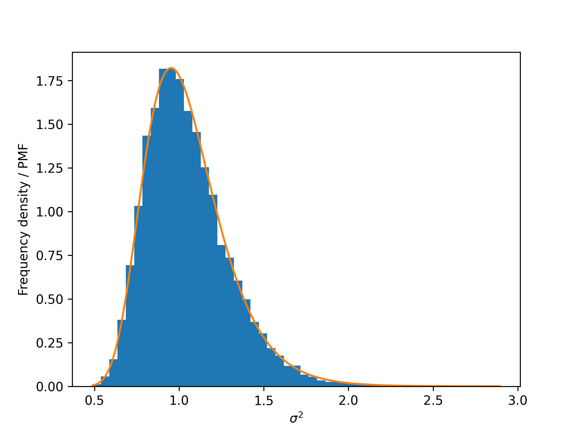
Suppose we wish to investigate the relationship between the normal-inverse-gamma distribution and the inverse gamma distribution.

import numpy as np
from scipy import stats
import matplotlib.pyplot as plt
rng = np.random.default_rng(527484872345)
mu, lmbda, a, b = 0, 1, 20, 20
norm_inv_gamma = stats.normal_inverse_gamma(mu, lmbda, a, b)
inv_gamma = stats.invgamma(a, scale=b)

✓

One approach is to compare the distribution of the `s2` elements of random variates against the PDF of an inverse gamma distribution.

_, s2 = norm_inv_gamma.rvs(size=10000, random_state=rng)
bins = np.linspace(s2.min(), s2.max(), 50)

✓

plt.hist(s2, bins=bins, density=True, label='Frequency density')

✗

s2 = np.linspace(s2.min(), s2.max(), 300)

✓

plt.plot(s2, inv_gamma.pdf(s2), label='PDF')
plt.xlabel(r'$\sigma^2$')
plt.ylabel('Frequency density / PMF')

✗

plt.show()

✓

Similarly, we can compare the marginal distribution of `s2` against an inverse gamma distribution.

from scipy.integrate import quad_vec
from scipy import integrate
s2 = np.linspace(0.5, 3, 6)
res = quad_vec(lambda x: norm_inv_gamma.pdf(x, s2), -np.inf, np.inf)[0]
np.allclose(res, inv_gamma.pdf(s2))

✓

The sample mean is comparable to the mean of the distribution.

x, s2 = norm_inv_gamma.rvs(size=10000, random_state=rng)

✓

x.mean(), s2.mean()

✗

norm_inv_gamma.mean()

✓

Similarly, for the variance:

x.var(ddof=1), s2.var(ddof=1)
norm_inv_gamma.var()

✓

Aliases

scipy.stats._multivariate.normal_inverse_gamma_gen