`scipy.stats._multivariate:vonmises_fisher_gen`

source: /scipy/stats/_multivariate.py :7025

Signature

class vonmises_fisher_gen ( seed = None )

Members

Summary

A von Mises-Fisher variable.

Extended Summary

The mu keyword specifies the mean direction vector. The kappa keyword specifies the concentration parameter.

Parameters

mu : array_like: Mean direction of the distribution. Must be a one-dimensional unit vector of norm 1.
kappa : float: Concentration parameter. Must be positive.
seed : {None, int, np.random.RandomState, np.random.Generator}, optional: Used for drawing random variates. If seed is None, the ~np.random.RandomState singleton is used. If seed is an int, a new RandomState instance is used, seeded with seed. If seed is already a RandomState or Generator instance, then that object is used. Default is None.

Methods

pdf(x, mu=None, kappa=1): Probability density function.
logpdf(x, mu=None, kappa=1): Log of the probability density function.
rvs(mu=None, kappa=1, size=1, random_state=None): Draw random samples from a von Mises-Fisher distribution.
entropy(mu=None, kappa=1): Compute the differential entropy of the von Mises-Fisher distribution.
fit(data): Fit a von Mises-Fisher distribution to data.

Notes

The von Mises-Fisher distribution is a directional distribution on the surface of the unit hypersphere. The probability density function of a unit vector $x$ is

f (x) = \frac{κ ^{d /2 - 1}}{( 2 π ) ^{d /2} I _{d /2 - 1} ( κ )} exp (κ μ^{T} x),

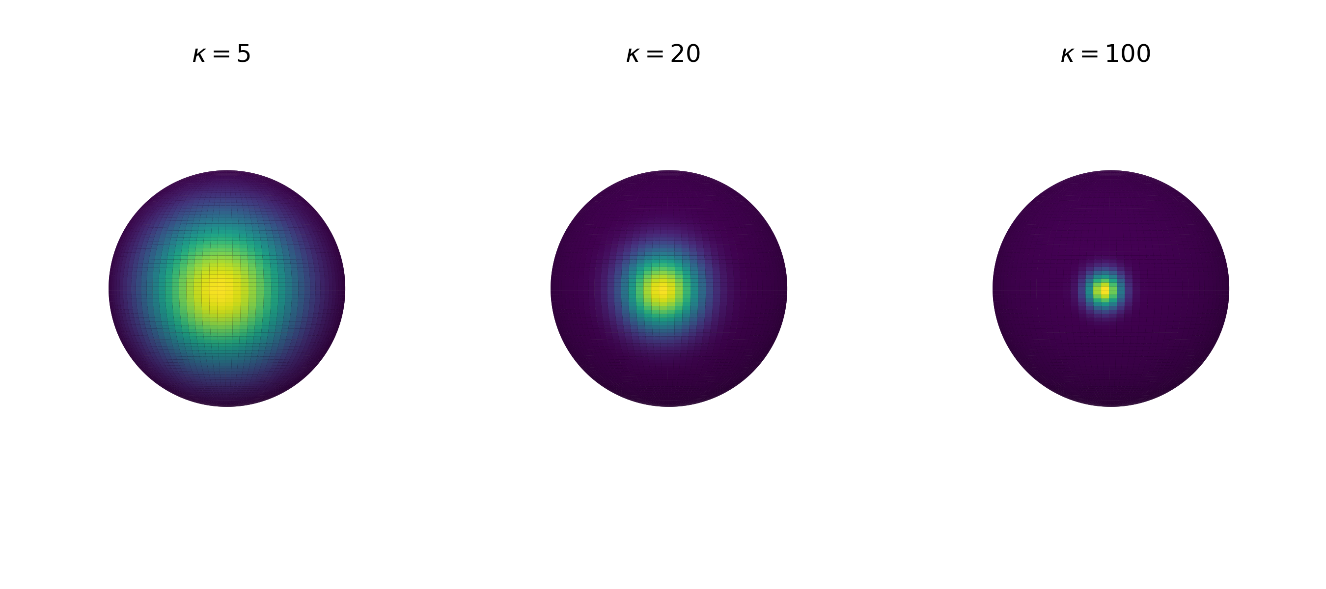
where $μ$ is the mean direction, $κ$ the concentration parameter, $d$ the dimension and $I$ the modified Bessel function of the first kind. As $μ$ represents a direction, it must be a unit vector or in other words, a point on the hypersphere: $μ \in S^{d - 1}$ . $κ$ is a concentration parameter, which means that it must be positive ( $κ > 0$ ) and that the distribution becomes more narrow with increasing $κ$ . In that sense, the reciprocal value $1/ κ$ resembles the variance parameter of the normal distribution.

The von Mises-Fisher distribution often serves as an analogue of the normal distribution on the sphere. Intuitively, for unit vectors, a useful distance measure is given by the angle $α$ between them. This is exactly what the scalar product $μ^{T} x = cos (α)$ in the von Mises-Fisher probability density function describes: the angle between the mean direction $μ$ and the vector $x$ . The larger the angle between them, the smaller the probability to observe $x$ for this particular mean direction $μ$ .

In dimensions 2 and 3, specialized algorithms are used for fast sampling ^[2], ^[3]. For dimensions of 4 or higher the rejection sampling algorithm described in ^[4] is utilized. This implementation is partially based on the geomstats package ^[5], ^[6].

Examples

**Visualization of the probability density** Plot the probability density in three dimensions for increasing concentration parameter. The density is calculated by the ``pdf`` method.

import numpy as np
import matplotlib.pyplot as plt
from scipy.stats import vonmises_fisher
from matplotlib.colors import Normalize
n_grid = 100
u = np.linspace(0, np.pi, n_grid)
v = np.linspace(0, 2 * np.pi, n_grid)
u_grid, v_grid = np.meshgrid(u, v)
vertices = np.stack([np.cos(v_grid) * np.sin(u_grid),
                     np.sin(v_grid) * np.sin(u_grid),
                     np.cos(u_grid)],
                    axis=2)
x = np.outer(np.cos(v), np.sin(u))
y = np.outer(np.sin(v), np.sin(u))
z = np.outer(np.ones_like(u), np.cos(u))
def plot_vmf_density(ax, x, y, z, vertices, mu, kappa):
    vmf = vonmises_fisher(mu, kappa)
    pdf_values = vmf.pdf(vertices)
    pdfnorm = Normalize(vmin=pdf_values.min(), vmax=pdf_values.max())
    ax.plot_surface(x, y, z, rstride=1, cstride=1,
                    facecolors=plt.cm.viridis(pdfnorm(pdf_values)),
                    linewidth=0)
    ax.set_aspect('equal')
    ax.view_init(azim=-130, elev=0)
    ax.axis('off')
    ax.set_title(rf"$\kappa={kappa}$")
fig, axes = plt.subplots(nrows=1, ncols=3, figsize=(9, 4),
                         subplot_kw={"projection": "3d"})
left, middle, right = axes
mu = np.array([-np.sqrt(0.5), -np.sqrt(0.5), 0])
plot_vmf_density(left, x, y, z, vertices, mu, 5)
plot_vmf_density(middle, x, y, z, vertices, mu, 20)
plot_vmf_density(right, x, y, z, vertices, mu, 100)
plt.subplots_adjust(top=1, bottom=0.0, left=0.0, right=1.0, wspace=0.)
plt.show()

✓

As we increase the concentration parameter, the points are getting more clustered together around the mean direction. **Sampling** Draw 5 samples from the distribution using the ``rvs`` method resulting in a 5x3 array.

rng = np.random.default_rng()
mu = np.array([0, 0, 1])
samples = vonmises_fisher(mu, 20).rvs(5, random_state=rng)

✓

samples

✗

These samples are unit vectors on the sphere :math:`S^2`. To verify, let us calculate their euclidean norms:

np.linalg.norm(samples, axis=1)

✓

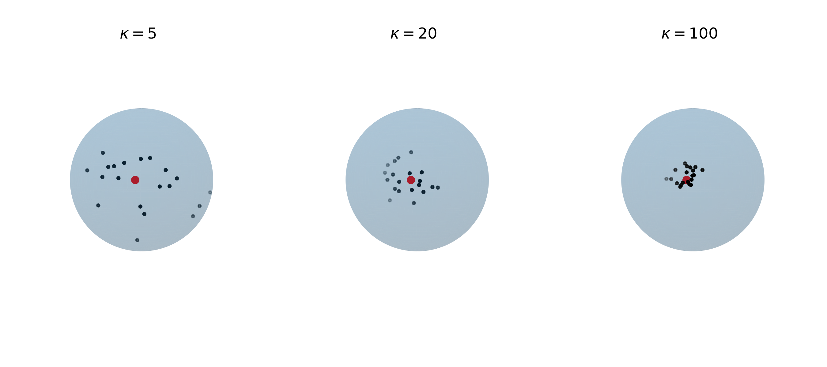
Plot 20 observations drawn from the von Mises-Fisher distribution for increasing concentration parameter :math:`\kappa`. The red dot highlights the mean direction :math:`\mu`.

def plot_vmf_samples(ax, x, y, z, mu, kappa):
    vmf = vonmises_fisher(mu, kappa)
    samples = vmf.rvs(20)
    ax.plot_surface(x, y, z, rstride=1, cstride=1, linewidth=0,
                    alpha=0.2)
    ax.scatter(samples[:, 0], samples[:, 1], samples[:, 2], c='k', s=5)
    ax.scatter(mu[0], mu[1], mu[2], c='r', s=30)
    ax.set_aspect('equal')
    ax.view_init(azim=-130, elev=0)
    ax.axis('off')
    ax.set_title(rf"$\kappa={kappa}$")
mu = np.array([-np.sqrt(0.5), -np.sqrt(0.5), 0])
fig, axes = plt.subplots(nrows=1, ncols=3,
                         subplot_kw={"projection": "3d"},
                         figsize=(9, 4))
left, middle, right = axes
plot_vmf_samples(left, x, y, z, mu, 5)
plot_vmf_samples(middle, x, y, z, mu, 20)
plot_vmf_samples(right, x, y, z, mu, 100)
plt.subplots_adjust(top=1, bottom=0.0, left=0.0,
                    right=1.0, wspace=0.)
plt.show()

✓

The plots show that with increasing concentration :math:`\kappa` the resulting samples are centered more closely around the mean direction. **Fitting the distribution parameters** The distribution can be fitted to data using the ``fit`` method returning the estimated parameters. As a toy example let's fit the distribution to samples drawn from a known von Mises-Fisher distribution.

mu, kappa = np.array([0, 0, 1]), 20
samples = vonmises_fisher(mu, kappa).rvs(1000, random_state=rng)
mu_fit, kappa_fit = vonmises_fisher.fit(samples)

✓

mu_fit, kappa_fit

✗

We see that the estimated parameters `mu_fit` and `kappa_fit` are very close to the ground truth parameters.

Aliases

scipy.stats._multivariate.vonmises_fisher_gen