bundles / scipy 2.0.0.dev0+git20260907.41eeb59 / scipy / signal / _waveforms / unit_impulse

function

`scipy.signal._waveforms:unit_impulse`

source: build-install/usr/lib/python3.14/site-packages/scipy/signal/_waveforms.py:592

Signature

def unit_impulse(shape, idx = None, dtype = <class 'float'>)

Summary

Unit impulse signal (discrete delta function) or unit basis vector.

Parameters

shape : int or tuple of int: Number of samples in the output (1-D), or a tuple that represents the shape of the output (N-D).
idx : None or int or tuple of int or 'mid', optional: Index at which the value is 1. If None, defaults to the 0th element. If idx='mid', the impulse will be centered at shape // 2 in all dimensions. If an int, the impulse will be at idx in all dimensions.
dtype : data-type, optional: The desired data-type for the array, e.g., numpy.int8. Default is numpy.float64.

Returns

y : ndarray: Output array containing an impulse signal.

Notes

In digital signal processing literature the unit impulse signal is often represented by the Kronecker delta. ^[1] I.e., a signal $u_{k} [n]$ , which is zero everywhere except being one at the $k$ -th sample, can be expressed as

u_{k} [n] = δ [n - k] \equiv δ_{n, k} .

Furthermore, the unit impulse is frequently interpreted as the discrete-time version of the continuous-time Dirac distribution. ^[2]

Examples

An impulse at the 0th element (:math:`\\delta[n]`):

from scipy import signal

✓

signal.unit_impulse(8)

✗

array([1., 0., 0., 0., 0., 0., 0., 0.])

Impulse offset by 2 samples (:math:`\\delta[n-2]`):

signal.unit_impulse(7, 2)

✗

array([0., 0., 1., 0., 0., 0., 0.])

2-dimensional impulse, centered:

signal.unit_impulse((3, 3), 'mid')

✗

array([[0., 0., 0.],
       [0., 1., 0.],
       [0., 0., 0.]])

Impulse at (2, 2), using broadcasting:

signal.unit_impulse((4, 4), 2)

✗

array([[0., 0., 0., 0.],
       [0., 0., 0., 0.],
       [0., 0., 1., 0.],
       [0., 0., 0., 0.]])

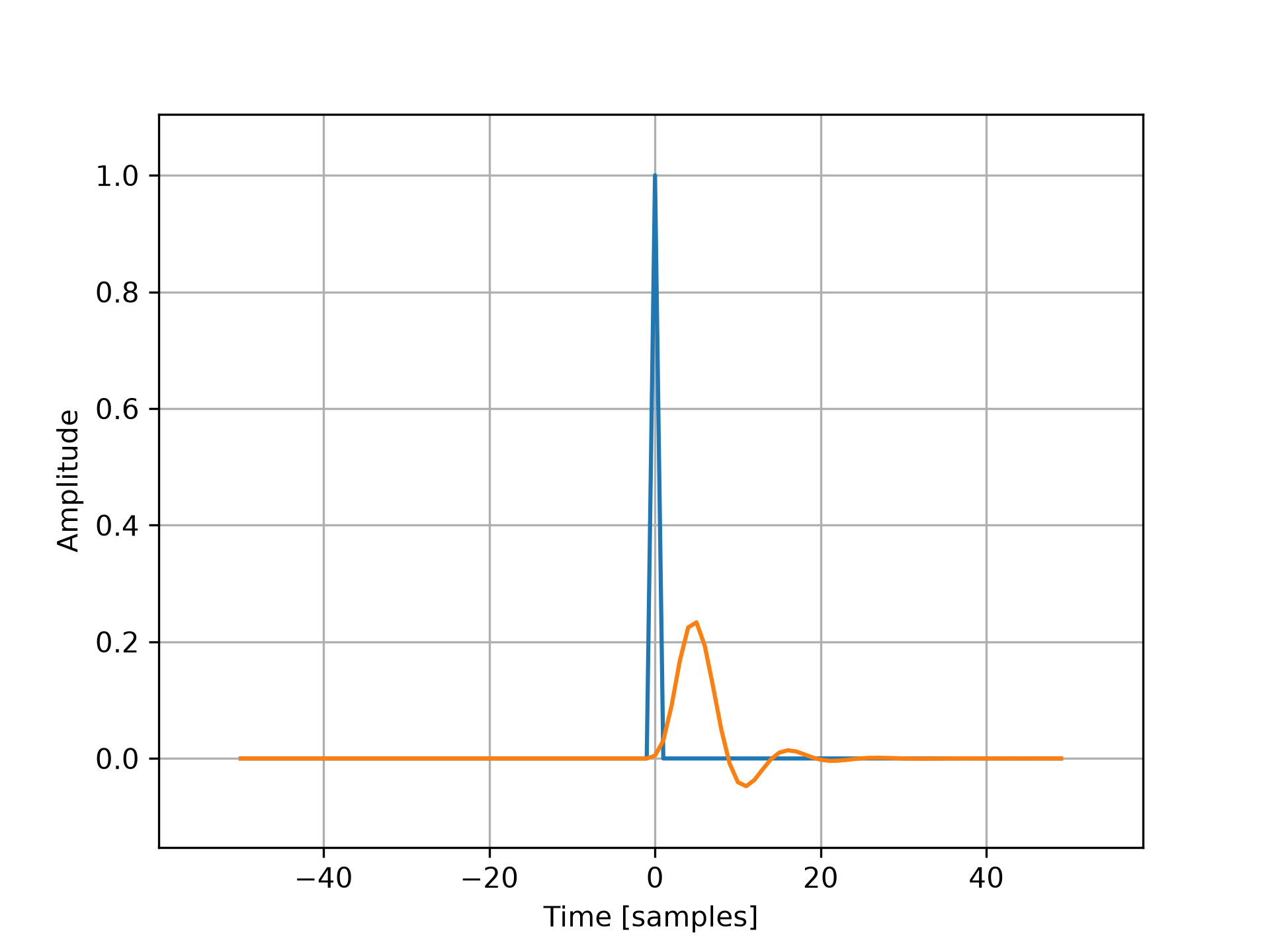
Plot the impulse response of a 4th-order Butterworth lowpass filter:

imp = signal.unit_impulse(100, 'mid')
b, a = signal.butter(4, 0.2)
response = signal.lfilter(b, a, imp)

✓

import numpy as np
import matplotlib.pyplot as plt

✓

plt.plot(np.arange(-50, 50), imp)
plt.plot(np.arange(-50, 50), response)

✗

[<matplotlib.lines.Line2D object at 0x7f3f68635a90>]

plt.margins(0.1, 0.1)

✓

plt.xlabel('Time [samples]')
plt.ylabel('Amplitude')

✗

Text(0, 0.5, 'Amplitude')

plt.grid(True)
plt.show()

✓