bundles / scipy 2.0.0.dev0+git20260907.41eeb59 / scipy / stats / _continuous_distns / studentized_range_gen

class

`scipy.stats._continuous_distns:studentized_range_gen`

source: build-install/usr/lib/python3.14/site-packages/scipy/stats/_continuous_distns.py:12289

Signature

class studentized_range_gen(momtype = 1, a = None, b = None, xtol = 1e-14, badvalue = None, name = None, longname = None, shapes = None, seed = None)

Members

Summary

A studentized range continuous random variable.

Extended Summary

%(before_notes)s

Notes

The probability density function for studentized_range is:

f (x; k, ν) = \frac{k ( k - 1 ) ν ^{ν /2}}{Γ ( ν /2 ) 2 ^{ν /2 - 1}} \int_{0}^{\infty} \int_{- \infty}^{\infty} s^{ν} e^{- ν s^{2} /2} ϕ (z) ϕ (s x + z) [Φ (s x + z) - Φ (z)]^{k - 2} d z d s

for $x \geq 0$ , $k > 1$ , and $ν > 0$ .

studentized_range takes k for $k$ and df for $ν$ as shape parameters.

When $ν$ exceeds 100,000, an asymptotic approximation (infinite degrees of freedom) is used to compute the cumulative distribution function ^[4] and probability distribution function.

%(after_notes)s

Examples

import numpy as np
from scipy.stats import studentized_range
import matplotlib.pyplot as plt
fig, ax = plt.subplots(1, 1)

✓

Display the probability density function (``pdf``):

k, df = 3, 10
x = np.linspace(studentized_range.ppf(0.01, k, df),
                studentized_range.ppf(0.99, k, df), 100)

✓

ax.plot(x, studentized_range.pdf(x, k, df),
        'r-', lw=5, alpha=0.6, label='studentized_range pdf')

✗

[<matplotlib.lines.Line2D object at 0x7f3f68548d70>]

Alternatively, the distribution object can be called (as a function) to fix the shape, location and scale parameters. This returns a "frozen" RV object holding the given parameters fixed. Freeze the distribution and display the frozen ``pdf``:

rv = studentized_range(k, df)

✓

ax.plot(x, rv.pdf(x), 'k-', lw=2, label='frozen pdf')

✗

[<matplotlib.lines.Line2D object at 0x7f3f6854aa50>]

Check accuracy of ``cdf`` and ``ppf``:

vals = studentized_range.ppf([0.001, 0.5, 0.999], k, df)
np.allclose([0.001, 0.5, 0.999], studentized_range.cdf(vals, k, df))

✓

True

Rather than using (``studentized_range.rvs``) to generate random variates, which is very slow for this distribution, we can approximate the inverse CDF using an interpolator, and then perform inverse transform sampling with this approximate inverse CDF. This distribution has an infinite but thin right tail, so we focus our attention on the leftmost 99.9 percent.

a, b = studentized_range.ppf([0, .999], k, df)

✓

a, b

✗

(np.float64(0.0), np.float64(7.41058083802341))

from scipy.interpolate import interp1d
rng = np.random.default_rng()
xs = np.linspace(a, b, 50)

✓

cdf = studentized_range.cdf(xs, k, df)
ppf = interp1d(cdf, xs, fill_value='extrapolate')

✗

r = ppf(rng.uniform(size=1000))

✓

And compare the histogram:

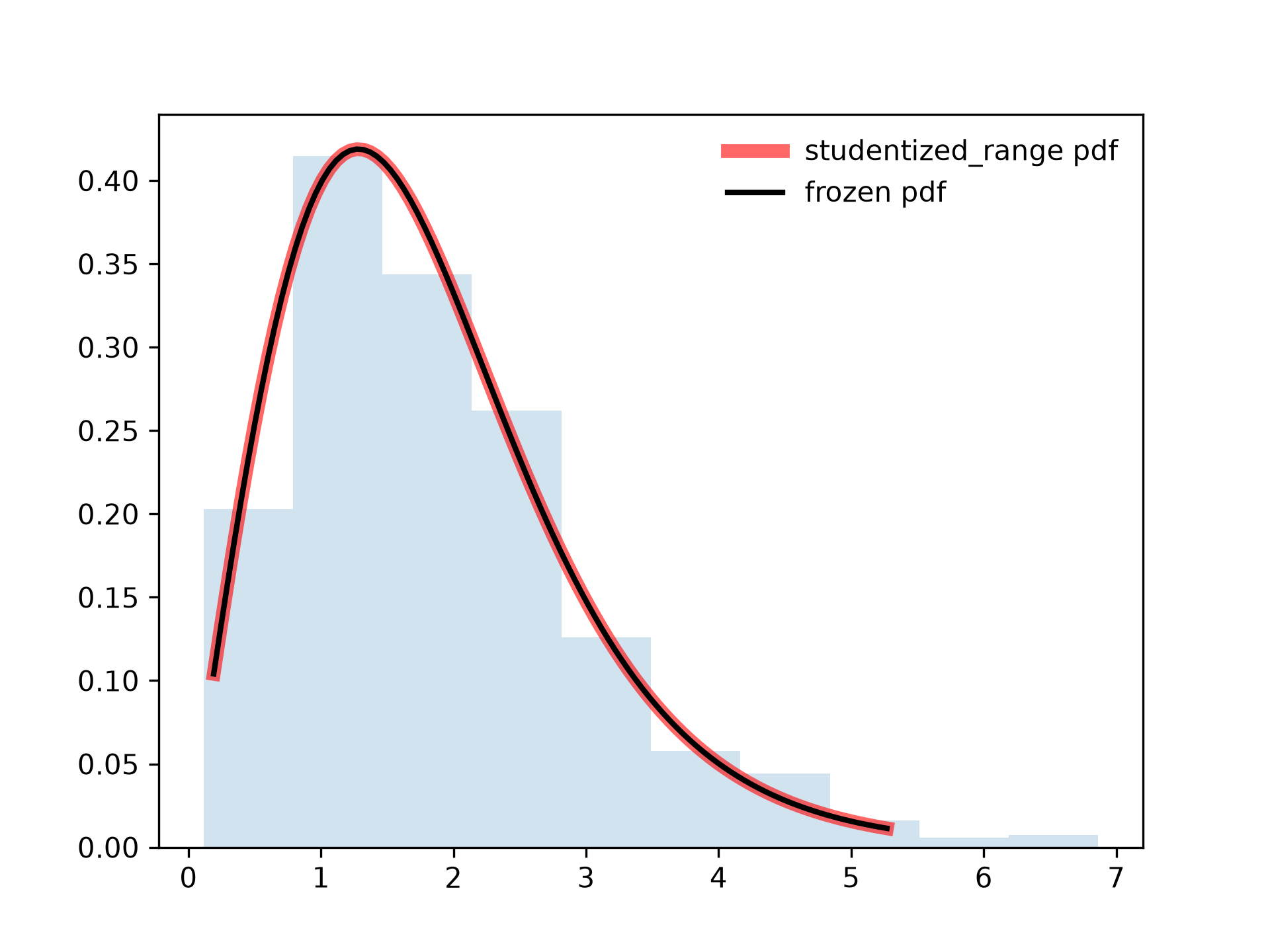
ax.hist(r, density=True, histtype='stepfilled', alpha=0.2)
ax.legend(loc='best', frameon=False)

✗

<matplotlib.legend.Legend object at 0x7f3f6854bb60>

plt.show()

✓

Aliases

scipy.stats._continuous_distns.studentized_range_gen