bundles / scipy latest / scipy / differentiate / _differentiate / derivative

function

`scipy.differentiate._differentiate:derivative`

source: /scipy/differentiate/_differentiate.py :65

Signature

   def     derivative (    f    ,    x    ,  * ,     args    =  ()   ,    tolerances    =  None   ,    maxiter    =  10   ,    order    =  8   ,    initial_step    =  0.5   ,    step_factor    =  2.0   ,    step_direction    =  0   ,    preserve_shape    =  False   ,    callback    =  None     )

Summary

Evaluate the derivative of an elementwise, real scalar function numerically.

Extended Summary

For each element of the output of f, derivative approximates the first derivative of f at the corresponding element of x using finite difference differentiation.

This function works elementwise when x, step_direction, and args contain (broadcastable) arrays.

Parameters

f : callable

The function whose derivative is desired. The signature must be

f(xi: ndarray, *argsi) -> ndarray

where each element of xi is a finite real number and argsi is a tuple, which may contain an arbitrary number of arrays that are broadcastable with xi. f must be an elementwise function: each scalar element f(xi)[j] must equal f(xi[j]) for valid indices j. It must not mutate the array xi or the arrays in argsi.

x : float array_like

Abscissae at which to evaluate the derivative. Must be broadcastable with args and step_direction.

args : tuple of array_like, optional

Additional positional array arguments to be passed to f. Arrays must be broadcastable with one another and the arrays of init. If the callable for which the root is desired requires arguments that are not broadcastable with x, wrap that callable with f such that f accepts only x and broadcastable *args.

tolerances : dictionary of floats, optional

Absolute and relative tolerances. Valid keys of the dictionary are:

atol - absolute tolerance on the derivative
rtol - relative tolerance on the derivative

Iteration will stop when res.error < atol + rtol * abs(res.df). The default atol is the smallest normal number of the appropriate dtype, and the default rtol is the square root of the precision of the appropriate dtype.

order : int, default: 8

The (positive integer) order of the finite difference formula to be used. Odd integers will be rounded up to the next even integer.

initial_step : float array_like, default: 0.5

The (absolute) initial step size for the finite difference derivative approximation.

step_factor : float, default: 2.0

The factor by which the step size is reduced in each iteration; i.e. the step size in iteration 1 is initial_step/step_factor. If step_factor < 1, subsequent steps will be greater than the initial step; this may be useful if steps smaller than some threshold are undesirable (e.g. due to subtractive cancellation error).

maxiter : int, default: 10

The maximum number of iterations of the algorithm to perform. See Notes.

step_direction : integer array_like

An array representing the direction of the finite difference steps (for use when x lies near to the boundary of the domain of the function.) Must be broadcastable with x and all args. Where 0 (default), central differences are used; where negative (e.g. -1), steps are non-positive; and where positive (e.g. 1), all steps are non-negative.

preserve_shape : bool, default: False

In the following, "arguments of f" refers to the array xi and any arrays within argsi. Let shape be the broadcasted shape of x and all elements of args (which is conceptually distinct from xi` and ``argsi passed into f).

When preserve_shape=False (default), f must accept arguments of any broadcastable shapes.
When preserve_shape=True, f must accept arguments of shape shape or shape + (n,), where (n,) is the number of abscissae at which the function is being evaluated.

In either case, for each scalar element xi[j] within xi, the array returned by f must include the scalar f(xi[j]) at the same index. Consequently, the shape of the output is always the shape of the input xi.

See Examples.

callback : callable, optional

An optional user-supplied function to be called before the first iteration and after each iteration. Called as callback(res), where res is a _RichResult similar to that returned by derivative (but containing the current iterate's values of all variables). If callback raises a StopIteration, the algorithm will terminate immediately and derivative will return a result. callback must not mutate res or its attributes.

Returns

res : _RichResult

An object similar to an instance of scipy.optimize.OptimizeResult with the following attributes. The descriptions are written as though the values will be scalars; however, if f returns an array, the outputs will be arrays of the same shape.

success: success
status: status
df: df
error: error
nit: nit
nfev: nfev
x: x

Notes

The implementation was inspired by jacobi ^[1], numdifftools ^[2], and DERIVEST ^[3], but the implementation follows the theory of Taylor series more straightforwardly (and arguably naively so). In the first iteration, the derivative is estimated using a finite difference formula of order order with maximum step size initial_step. Each subsequent iteration, the maximum step size is reduced by step_factor, and the derivative is estimated again until a termination condition is reached. The error estimate is the magnitude of the difference between the current derivative approximation and that of the previous iteration.

The stencils of the finite difference formulae are designed such that abscissae are "nested": after f is evaluated at order + 1 points in the first iteration, f is evaluated at only two new points in each subsequent iteration; order - 1 previously evaluated function values required by the finite difference formula are reused, and two function values (evaluations at the points furthest from x) are unused.

Step sizes are absolute. When the step size is small relative to the magnitude of x, precision is lost; for example, if x is 1e20, the default initial step size of 0.5 cannot be resolved. Accordingly, consider using larger initial step sizes for large magnitudes of x.

The default tolerances are challenging to satisfy at points where the true derivative is exactly zero. If the derivative may be exactly zero, consider specifying an absolute tolerance (e.g. atol=1e-12) to improve convergence.

Array API Standard Support

derivative has experimental support for Python Array API Standard compatible backends in addition to NumPy. Please consider testing these features by setting an environment variable SCIPY_ARRAY_API=1 and providing CuPy, PyTorch, JAX, or Dask arrays as array arguments. The following combinations of backend and device (or other capability) are supported.

====================  ====================  ====================
Library               CPU                   GPU
====================  ====================  ====================
NumPy                 ✅                     n/a                 
CuPy                  n/a                   ✅                   
PyTorch               ✅                     ✅                   
JAX                   ⚠️ no JIT             ⚠️ no JIT           
Dask                  ⛔                     n/a                 
====================  ====================  ====================

See dev-arrayapi for more information.

Examples

Evaluate the derivative of ``np.exp`` at several points ``x``.

import numpy as np
from scipy.differentiate import derivative
f = np.exp
df = np.exp  # true derivative
x = np.linspace(1, 2, 5)
res = derivative(f, x)

✓

res.df  # approximation of the derivative
res.error  # estimate of the error
abs(res.df - df(x))  # true error

✗

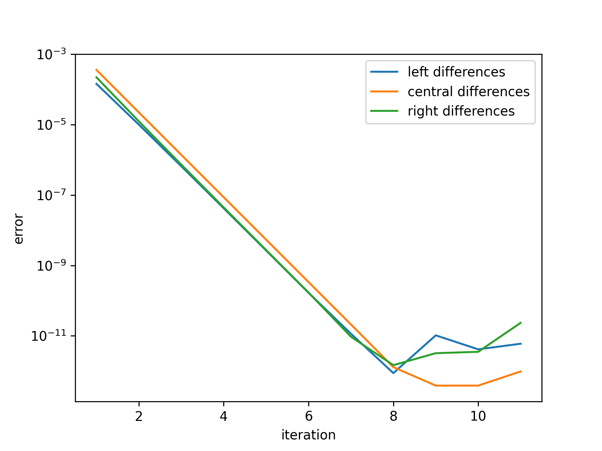
Show the convergence of the approximation as the step size is reduced. Each iteration, the step size is reduced by `step_factor`, so for sufficiently small initial step, each iteration reduces the error by a factor of ``1/step_factor**order`` until finite precision arithmetic inhibits further improvement.

import matplotlib.pyplot as plt
iter = list(range(1, 12))  # maximum iterations
hfac = 2  # step size reduction per iteration
hdir = [-1, 0, 1]  # compare left-, central-, and right- steps
order = 4  # order of differentiation formula
x = 1
ref = df(x)
errors = []  # true error
for i in iter:
    res = derivative(f, x, maxiter=i, step_factor=hfac,
                     step_direction=hdir, order=order,
                     # prevent early termination
                     tolerances=dict(atol=0, rtol=0))
    errors.append(abs(res.df - ref))
errors = np.array(errors)

✓

plt.semilogy(iter, errors[:, 0], label='left differences')
plt.semilogy(iter, errors[:, 1], label='central differences')
plt.semilogy(iter, errors[:, 2], label='right differences')
plt.xlabel('iteration')
plt.ylabel('error')
plt.legend()

✗

plt.show()

✓

(errors[1, 1] / errors[0, 1], 1 / hfac**order)

✗

The implementation is vectorized over `x`, `step_direction`, and `args`. The function is evaluated once before the first iteration to perform input validation and standardization, and once per iteration thereafter.

def f(x, p):
    f.nit += 1
    return x**p
f.nit = 0
def df(x, p):
    return p*x**(p-1)
x = np.arange(1, 5)
p = np.arange(1, 6).reshape((-1, 1))
hdir = np.arange(-1, 2).reshape((-1, 1, 1))
res = derivative(f, x, args=(p,), step_direction=hdir, maxiter=1)
np.allclose(res.df, df(x, p))
res.df.shape
f.nit

✓

By default, `preserve_shape` is False, and therefore the callable `f` may be called with arrays of any broadcastable shapes. For example:

shapes = []
def f(x, c):
   shape = np.broadcast_shapes(x.shape, c.shape)
   shapes.append(shape)
   return np.sin(c*x)
c = [1, 5, 10, 20]
res = derivative(f, 0, args=(c,))
shapes

✓

To understand where these shapes are coming from - and to better understand how `derivative` computes accurate results - note that higher values of ``c`` correspond with higher frequency sinusoids. The higher frequency sinusoids make the function's derivative change faster, so more function evaluations are required to achieve the target accuracy:

res.nfev

✓

The initial ``shape``, ``(4,)``, corresponds with evaluating the function at a single abscissa and all four frequencies; this is used for input validation and to determine the size and dtype of the arrays that store results. The next shape corresponds with evaluating the function at an initial grid of abscissae and all four frequencies. Successive calls to the function evaluate the function at two more abscissae, increasing the effective order of the approximation by two. However, in later function evaluations, the function is evaluated at fewer frequencies because the corresponding derivative has already converged to the required tolerance. This saves function evaluations to improve performance, but it requires the function to accept arguments of any shape. "Vector-valued" functions are unlikely to satisfy this requirement. For example, consider

def f(x):
   return [x, np.sin(3*x), x+np.sin(10*x), np.sin(20*x)*(x-1)**2]

✓

This integrand is not compatible with `derivative` as written; for instance, the shape of the output will not be the same as the shape of ``x``. Such a function *could* be converted to a compatible form with the introduction of additional parameters, but this would be inconvenient. In such cases, a simpler solution would be to use `preserve_shape`.

shapes = []
def f(x):
    shapes.append(x.shape)
    x0, x1, x2, x3 = x
    return [x0, np.sin(3*x1), x2+np.sin(10*x2), np.sin(20*x3)*(x3-1)**2]
x = np.zeros(4)
res = derivative(f, x, preserve_shape=True)
shapes

✓

Here, the shape of ``x`` is ``(4,)``. With ``preserve_shape=True``, the function may be called with argument ``x`` of shape ``(4,)`` or ``(4, n)``, and this is what we observe.

`scipy.differentiate._differentiate:derivative`

Signature

Summary

Extended Summary

Parameters

Returns

Notes

Examples

See also

Aliases

Referenced by

This package