`scipy.fft._fftlog:ifht`

source: build-install/usr/lib/python3.14/site-packages/scipy/fft/_fftlog.py:217

Signature

def ifht(A, dln, mu, offset = 0.0, bias = 0.0)

Summary

Compute the inverse fast Hankel transform.

Extended Summary

Computes the discrete inverse Hankel transform of a logarithmically spaced periodic sequence. This is the inverse operation to fht.

Parameters

A : array_like (..., n): Real periodic input array, uniformly logarithmically spaced. For multidimensional input, the transform is performed over the last axis.
dln : float: Uniform logarithmic spacing of the input array.
mu : float: Order of the Hankel transform, any positive or negative real number.
offset : float, optional: Offset of the uniform logarithmic spacing of the output array.
bias : float, optional: Exponent of power law bias, any positive or negative real number.

Returns

a : array_like (..., n): The transformed output array, which is real, periodic, uniformly logarithmically spaced, and of the same shape as the input array.

Notes

This function computes a discrete version of the Hankel transform

a (r) = \int_{0}^{\infty} A (k) J_{μ} (k r) r d k,

where $J_{μ}$ is the Bessel function of order $μ$ . The index $μ$ may be any real number, positive or negative. Note that the numerical inverse Hankel transform uses an integrand of $r d k$ , while the mathematical inverse Hankel transform is commonly defined using $k d k$ .

See fht for further details.

Examples

import numpy as np
import matplotlib.pyplot as plt
from scipy import fft
from scipy.special import jv

✓

Generate sample data ``A`` and evaluation points ``k`` for the Hankel transform of a signal.

k = np.logspace(-1, 1, 300)
A = np.zeros_like(k)
A[240] = 20

✓

Calculate the logarithmic spacing of the elements in ``A`` and perform a second-order inverse Hankel transform on the sample data.

dln = np.log(k[1]/k[0])
a = fft.ifht(A, dln, mu=2)

✓

Calculate the evaluation points for the transformed data ``a``. ``ifht`` calculates evaluation points ``r`` such that ``k * r`` is constant for each ``k`` and then returns the transformed data in ascending order of evaluation points. To calculate the evaluation points in ascending order, flip the order of ``k`` in the equation for ``r``.

r = 1/np.flip(k)

✓

Compare ``a`` with the kernel function corresponding to ``k[240]``.

a_f = jv(2, k[240]*r)*r
fig, ax = plt.subplots()

✓

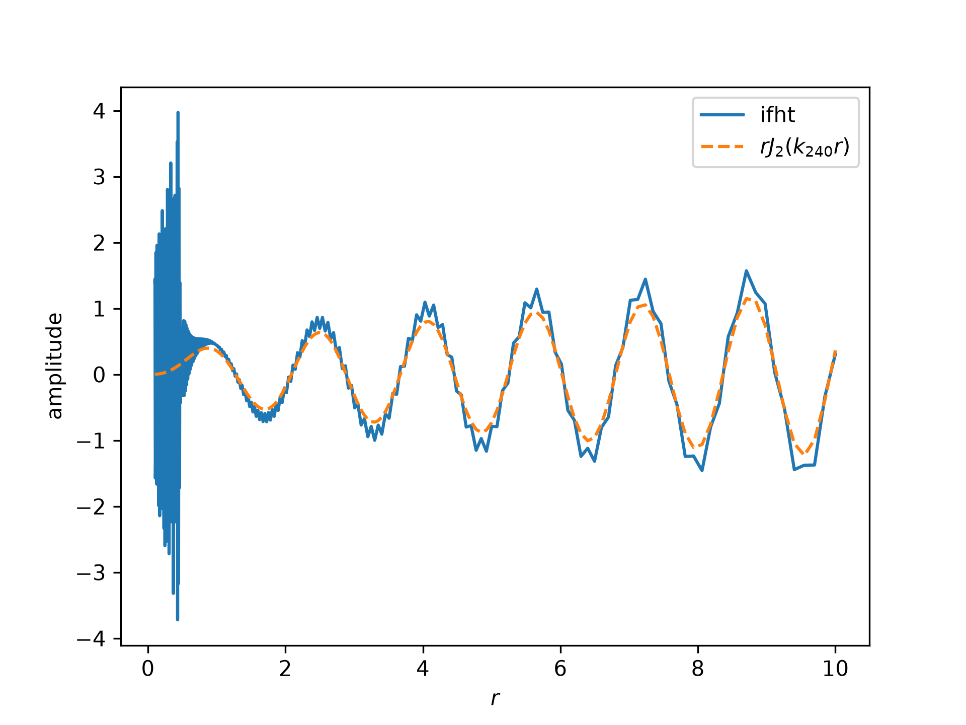
ax.plot(r, a, label="ifht")
ax.plot(r, a_f, "--", label=r"$r J_2(k_{240} r)$")
ax.set_xlabel(r"$r$")
ax.set_ylabel("amplitude")
ax.legend()

✗

<matplotlib.legend.Legend object at 0x7f3f687c9fd0>

plt.show()

✓

The plot shows that, for larger values of ``r``, the inverse Hankel transform follows the kernel function closely.

`scipy.fft._fftlog:ifht`

Signature

Summary

Extended Summary

Parameters

Returns

Notes

Examples

See also

Aliases

Referenced by

This package