bundles / scipy latest / scipy / integrate / _bvp / solve_bvp

function

`scipy.integrate._bvp:solve_bvp`

source: /scipy/integrate/_bvp.py :712

Signature

   def     solve_bvp (    fun    ,    bc    ,    x    ,    y    ,    p    =  None   ,    S    =  None   ,    fun_jac    =  None   ,    bc_jac    =  None   ,    tol    =  0.001   ,    max_nodes    =  1000   ,    verbose    =  0   ,    bc_tol    =  None     )

Summary

Solve a boundary value problem for a system of ODEs.

Extended Summary

This function numerically solves a first order system of ODEs subject to two-point boundary conditions

dy / dx = f(x, y, p) + S * y / (x - a), a <= x <= b
bc(y(a), y(b), p) = 0

Here x is a 1-D independent variable, y(x) is an n-D vector-valued function and p is a k-D vector of unknown parameters which is to be found along with y(x). For the problem to be determined, there must be n + k boundary conditions, i.e., bc must be an (n + k)-D function.

The last singular term on the right-hand side of the system is optional. It is defined by an n-by-n matrix S, such that the solution must satisfy S y(a) = 0. This condition will be forced during iterations, so it must not contradict boundary conditions. See ^[2] for the explanation how this term is handled when solving BVPs numerically.

Problems in a complex domain can be solved as well. In this case, y and p are considered to be complex, and f and bc are assumed to be complex-valued functions, but x stays real. Note that f and bc must be complex differentiable (satisfy Cauchy-Riemann equations ^[4]), otherwise you should rewrite your problem for real and imaginary parts separately. To solve a problem in a complex domain, pass an initial guess for y with a complex data type (see below).

Parameters

fun : callable

Right-hand side of the system. The calling signature is fun(x, y), or fun(x, y, p) if parameters are present. All arguments are ndarray: x with shape (m,), y with shape (n, m), meaning that y[:, i] corresponds to x[i], and p with shape (k,). The return value must be an array with shape (n, m) and with the same layout as y.

bc : callable

Function evaluating residuals of the boundary conditions. The calling signature is bc(ya, yb), or bc(ya, yb, p) if parameters are present. All arguments are ndarray: ya and yb with shape (n,), and p with shape (k,). The return value must be an array with shape (n + k,).

x : array_like, shape (m,)

Initial mesh. Must be a strictly increasing sequence of real numbers with x[0]=a and x[-1]=b.

y : array_like, shape (n, m)

Initial guess for the function values at the mesh nodes, ith column corresponds to x[i]. For problems in a complex domain pass y with a complex data type (even if the initial guess is purely real).

p : array_like with shape (k,) or None, optional

Initial guess for the unknown parameters. If None (default), it is assumed that the problem doesn't depend on any parameters.

S : array_like with shape (n, n) or None

Matrix defining the singular term. If None (default), the problem is solved without the singular term.

fun_jac : callable or None, optional

Function computing derivatives of f with respect to y and p. The calling signature is fun_jac(x, y), or fun_jac(x, y, p) if parameters are present. The return must contain 1 or 2 elements in the following order:

df_dyarray_like with shape (n, n, m), where an element (i, j, q) equals to d f_i(x_q, y_q, p) / d (y_q)_j.
df_dparray_like with shape (n, k, m), where an element (i, j, q) equals to d f_i(x_q, y_q, p) / d p_j.

Here q numbers nodes at which x and y are defined, whereas i and j number vector components. If the problem is solved without unknown parameters, df_dp should not be returned.

If fun_jac is None (default), the derivatives will be estimated by the forward finite differences.

bc_jac : callable or None, optional

Function computing derivatives of bc with respect to ya, yb, and p. The calling signature is bc_jac(ya, yb), or bc_jac(ya, yb, p) if parameters are present. The return must contain 2 or 3 elements in the following order:

dbc_dyaarray_like with shape (n, n), where an element (i, j) equals to d bc_i(ya, yb, p) / d ya_j.
dbc_dybarray_like with shape (n, n), where an element (i, j) equals to d bc_i(ya, yb, p) / d yb_j.
dbc_dparray_like with shape (n, k), where an element (i, j) equals to d bc_i(ya, yb, p) / d p_j.

If the problem is solved without unknown parameters, dbc_dp should not be returned.

If bc_jac is None (default), the derivatives will be estimated by the forward finite differences.

tol : float, optional

Desired tolerance of the solution. If we define r = y' - f(x, y), where y is the found solution, then the solver tries to achieve on each mesh interval norm(r / (1 + abs(f)) < tol, where norm is estimated in a root mean squared sense (using a numerical quadrature formula). Default is 1e-3.

max_nodes : int, optional

Maximum allowed number of the mesh nodes. If exceeded, the algorithm terminates. Default is 1000.

verbose : {0, 1, 2}, optional

Level of algorithm's verbosity:

0 (default)work silently.
1display a termination report.
2display progress during iterations.

bc_tol : float, optional

Desired absolute tolerance for the boundary condition residuals: bc value should satisfy abs(bc) < bc_tol component-wise. Equals to tol by default. Up to 10 iterations are allowed to achieve this tolerance.

Returns

: Bunch object with the following fields defined:

sol : PPoly

Found solution for y as scipy.interpolate.PPoly instance, a C1 continuous cubic spline.

p : ndarray or None, shape (k,)

Found parameters. None, if the parameters were not present in the problem.

x : ndarray, shape (m,)

Nodes of the final mesh.

y : ndarray, shape (n, m)

Solution values at the mesh nodes.

yp : ndarray, shape (n, m)

Solution derivatives at the mesh nodes.

rms_residuals : ndarray, shape (m - 1,)

RMS values of the relative residuals over each mesh interval (see the description of tol parameter).

niter : int

Number of completed iterations.

status : int

Reason for algorithm termination:

0: The algorithm converged to the desired accuracy.
1: The maximum number of mesh nodes is exceeded.
2: A singular Jacobian encountered when solving the collocation system.

message : string

Verbal description of the termination reason.

success : bool

True if the algorithm converged to the desired accuracy (status=0).

Notes

This function implements a 4th order collocation algorithm with the control of residuals similar to ^[1]. A collocation system is solved by a damped Newton method with an affine-invariant criterion function as described in ^[3].

Note that in ^[1] integral residuals are defined without normalization by interval lengths. So, their definition is different by a multiplier of h**0.5 (h is an interval length) from the definition used here.

Array API Standard Support

solve_bvp has experimental support for Python Array API Standard compatible backends in addition to NumPy. Please consider testing these features by setting an environment variable SCIPY_ARRAY_API=1 and providing CuPy, PyTorch, JAX, or Dask arrays as array arguments. The following combinations of backend and device (or other capability) are supported.

====================  ====================  ====================
Library               CPU                   GPU
====================  ====================  ====================
NumPy                 ✅                     n/a                 
CuPy                  n/a                   ⛔                   
PyTorch               ⛔                     ⛔                   
JAX                   ⛔                     ⛔                   
Dask                  ⛔                     n/a                 
====================  ====================  ====================

See dev-arrayapi for more information.

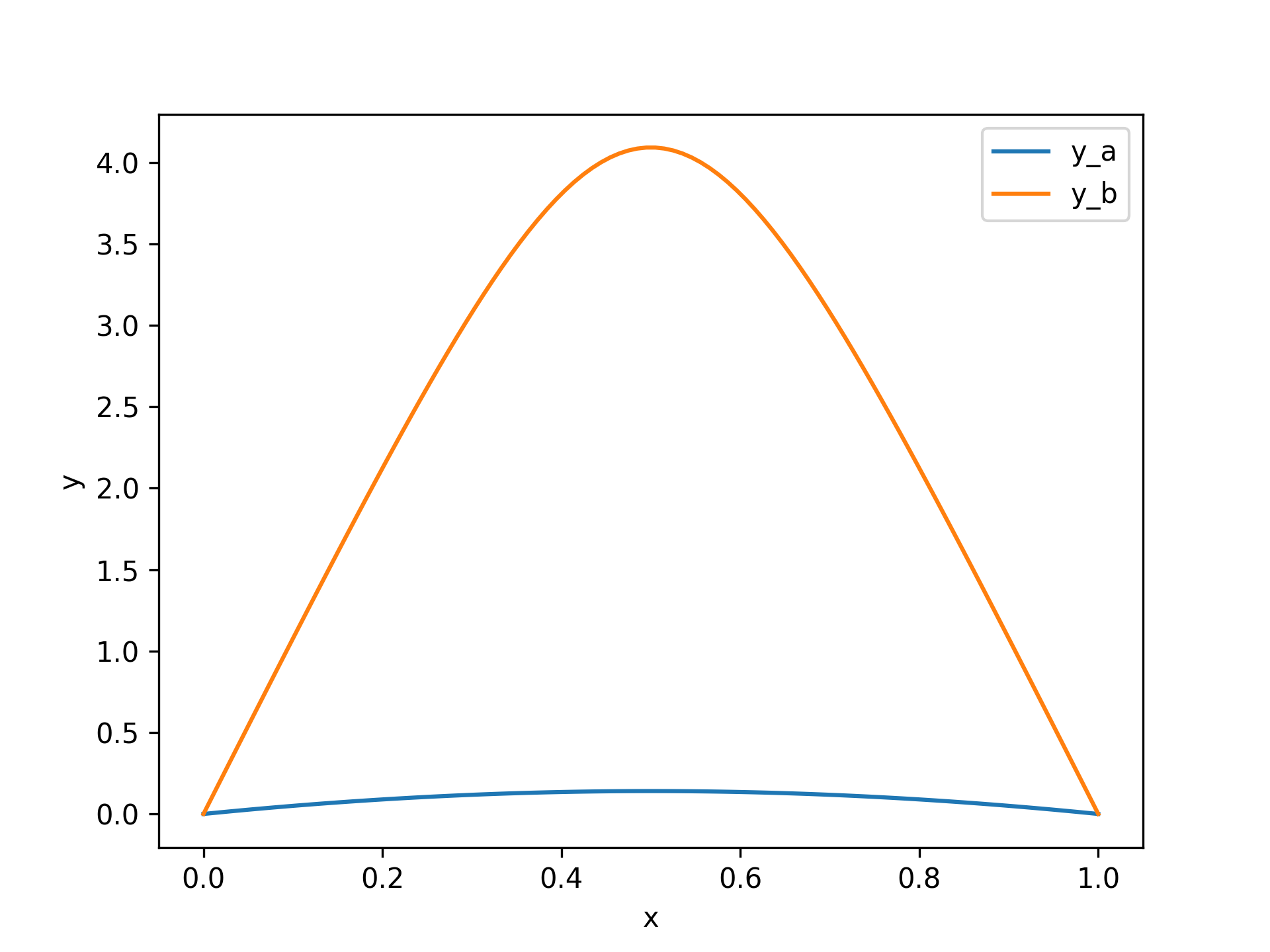
Examples

In the first example, we solve Bratu's problem:: y'' + k * exp(y) = 0 y(0) = y(1) = 0 for k = 1. We rewrite the equation as a first-order system and implement its right-hand side evaluation:: y1' = y2 y2' = -exp(y1)

import numpy as np
def fun(x, y):
    return np.vstack((y[1], -np.exp(y[0])))

✓

Implement evaluation of the boundary condition residuals:

def bc(ya, yb):
    return np.array([ya[0], yb[0]])

✓

Define the initial mesh with 5 nodes:

x = np.linspace(0, 1, 5)

✓

This problem is known to have two solutions. To obtain both of them, we use two different initial guesses for y. We denote them by subscripts a and b.

y_a = np.zeros((2, x.size))
y_b = np.zeros((2, x.size))
y_b[0] = 3

✓

Now we are ready to run the solver.

from scipy.integrate import solve_bvp
res_a = solve_bvp(fun, bc, x, y_a)
res_b = solve_bvp(fun, bc, x, y_b)

✓

Let's plot the two found solutions. We take an advantage of having the solution in a spline form to produce a smooth plot.

x_plot = np.linspace(0, 1, 100)
y_plot_a = res_a.sol(x_plot)[0]
y_plot_b = res_b.sol(x_plot)[0]
import matplotlib.pyplot as plt

✓

plt.plot(x_plot, y_plot_a, label='y_a')
plt.plot(x_plot, y_plot_b, label='y_b')
plt.legend()
plt.xlabel("x")
plt.ylabel("y")

✗

plt.show()

✓

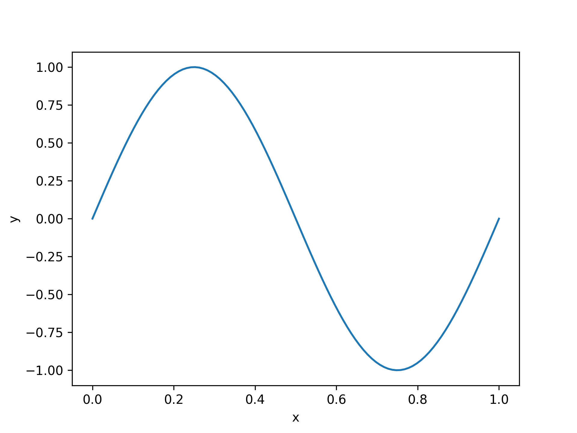
We see that the two solutions have similar shape, but differ in scale significantly. In the second example, we solve a simple Sturm-Liouville problem:: y'' + k**2 * y = 0 y(0) = y(1) = 0 It is known that a non-trivial solution y = A * sin(k * x) is possible for k = pi * n, where n is an integer. To establish the normalization constant A = 1 we add a boundary condition:: y'(0) = k Again, we rewrite our equation as a first-order system and implement its right-hand side evaluation:: y1' = y2 y2' = -k**2 * y1

def fun(x, y, p):
    k = p[0]
    return np.vstack((y[1], -k**2 * y[0]))

✓

Note that parameters p are passed as a vector (with one element in our case). Implement the boundary conditions:

def bc(ya, yb, p):
    k = p[0]
    return np.array([ya[0], yb[0], ya[1] - k])

✓

Set up the initial mesh and guess for y. We aim to find the solution for k = 2 * pi, to achieve that we set values of y to approximately follow sin(2 * pi * x):

x = np.linspace(0, 1, 5)
y = np.zeros((2, x.size))
y[0, 1] = 1
y[0, 3] = -1

✓

Run the solver with 6 as an initial guess for k.

sol = solve_bvp(fun, bc, x, y, p=[6])

✓

We see that the found k is approximately correct:

sol.p[0]

✗

And, finally, plot the solution to see the anticipated sinusoid:

x_plot = np.linspace(0, 1, 100)
y_plot = sol.sol(x_plot)[0]

✓

plt.plot(x_plot, y_plot)
plt.xlabel("x")
plt.ylabel("y")

✗

plt.show()

✓