bundles / scipy latest / scipy / interpolate / _rbfinterp / RBFInterpolator
class
scipy.interpolate._rbfinterp:RBFInterpolator
Signature
class RBFInterpolator ( y , d , neighbors = None , smoothing = 0.0 , kernel = thin_plate_spline , epsilon = None , degree = None ) Members
Summary
Radial basis function interpolator in N ≥ 1 dimensions.
Parameters
y: (npoints, ndims) array_like2-D array of data point coordinates.
d: (npoints, ...) array_likeN-D array of data values at
y. The length ofdalong the first axis must be equal to the length ofy. Unlike some interpolators, the interpolation axis cannot be changed.neighbors: int, optionalIf specified, the value of the interpolant at each evaluation point will be computed using only this many nearest data points. All the data points are used by default.
smoothing: float or (npoints, ) array_like, optionalSmoothing parameter. The interpolant perfectly fits the data when this is set to 0. For large values, the interpolant approaches a least squares fit of a polynomial with the specified degree. Default is 0.
kernel: str, optionalType of RBF. This should be one of
'linear'
-r'thin_plate_spline'
r**2 * log(r)'cubic'
r**3'quintic'
-r**5'multiquadric'
-sqrt(1 + r**2)'inverse_multiquadric'
1/sqrt(1 + r**2)'inverse_quadratic'
1/(1 + r**2)'gaussian'
exp(-r**2)
Default is 'thin_plate_spline'.
epsilon: float, optionalShape parameter that scales the input to the RBF. If
kernelis 'linear', 'thin_plate_spline', 'cubic', or 'quintic', this defaults to 1 and can be ignored because it has the same effect as scaling the smoothing parameter. Otherwise, this must be specified.degree: int, optionalDegree of the added polynomial. For some RBFs the interpolant may not be well-posed if the polynomial degree is too small. Those RBFs and their corresponding minimum degrees are
'multiquadric'0
'linear'0
'thin_plate_spline'1
'cubic'1
'quintic'2
The default value is the minimum degree for
kernelor 0 if there is no minimum degree. Set this to -1 for no added polynomial.
Notes
An RBF is a scalar valued function in N-dimensional space whose value at can be expressed in terms of , where is the center of the RBF.
An RBF interpolant for the vector of data values , which are from locations , is a linear combination of RBFs centered at plus a polynomial with a specified degree. The RBF interpolant is written as
where is a matrix of RBFs with centers at evaluated at the points , and is a matrix of monomials, which span polynomials with the specified degree, evaluated at . The coefficients and are the solution to the linear equations
and
where is a non-negative smoothing parameter that controls how well we want to fit the data. The data are fit exactly when the smoothing parameter is 0.
The above system is uniquely solvable if the following requirements are met:
must have full column rank. always has full column rank when
degreeis -1 or 0. Whendegreeis 1, has full column rank if the data point locations are not all collinear (N=2), coplanar (N=3), etc.If
kernelis 'multiquadric', 'linear', 'thin_plate_spline', 'cubic', or 'quintic', thendegreemust not be lower than the minimum value listed above.If
smoothingis 0, then each data point location must be distinct.
When using an RBF that is not scale invariant ('multiquadric', 'inverse_multiquadric', 'inverse_quadratic', or 'gaussian'), an appropriate shape parameter must be chosen (e.g., through cross validation). Smaller values for the shape parameter correspond to wider RBFs. The problem can become ill-conditioned or singular when the shape parameter is too small.
The memory required to solve for the RBF interpolation coefficients increases quadratically with the number of data points, which can become impractical when interpolating more than about a thousand data points. To overcome memory limitations for large interpolation problems, the neighbors argument can be specified to compute an RBF interpolant for each evaluation point using only the nearest data points.
Array API Standard Support
RBFInterpolator has experimental support for Python Array API Standard compatible backends in addition to NumPy. Please consider testing these features by setting an environment variable SCIPY_ARRAY_API=1 and providing CuPy, PyTorch, JAX, or Dask arrays as array arguments. The following combinations of backend and device (or other capability) are supported.
====================  ====================  ====================
Library               CPU                   GPU
====================  ====================  ====================
NumPy                 ✅                     n/a
CuPy                  n/a                   ✅
PyTorch               ✅                     ✅
JAX                   ✅                     ✅
Dask                  ⛔                     n/a
====================  ====================  ====================
Only the default neighbors=None is Array API compatible. If a non-default value of neighbors is given, the behavior is NumPy -only.
See dev-arrayapi for more information.
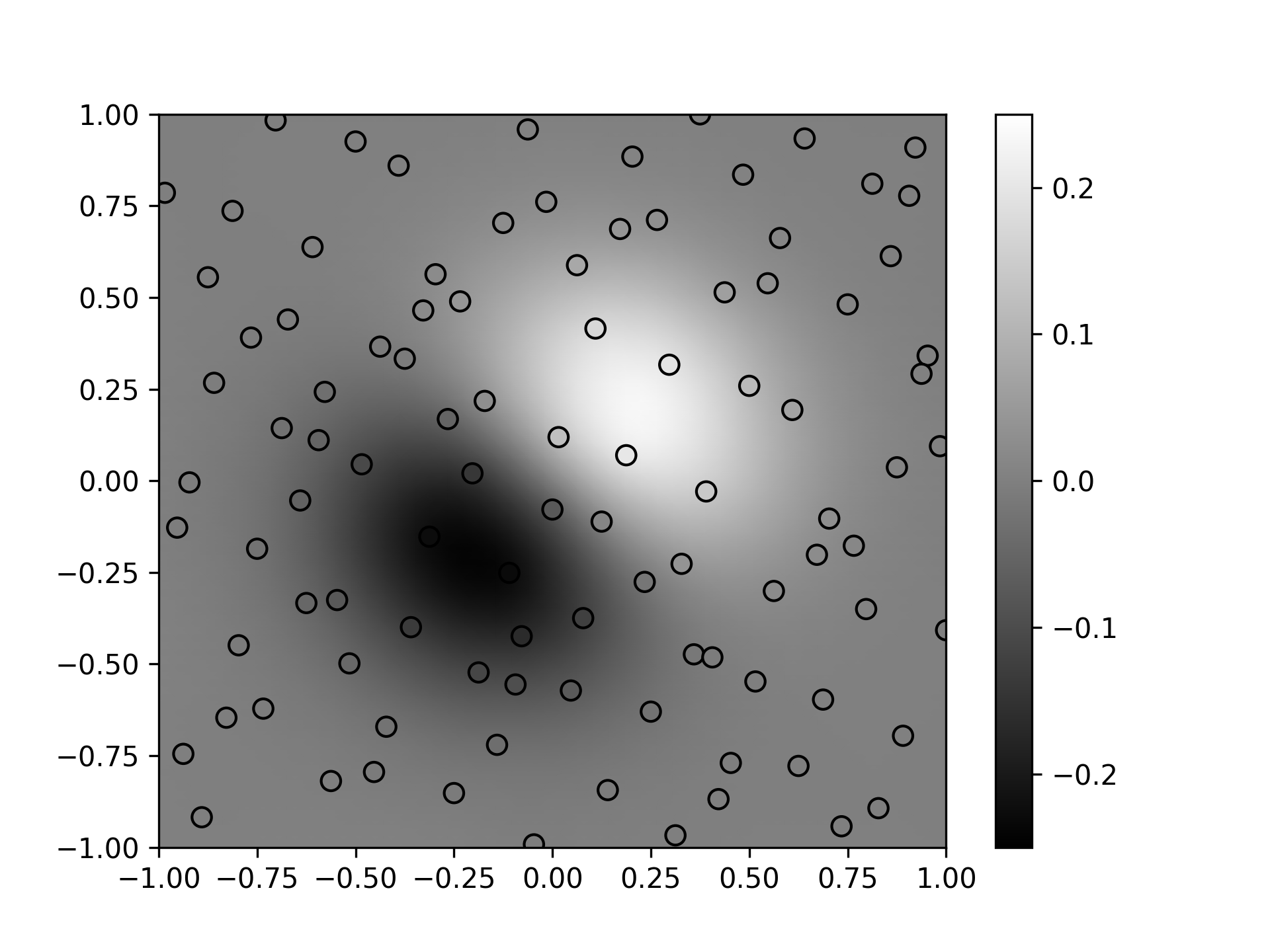
Examples
Demonstrate interpolating scattered data to a grid in 2-D.import numpy as np import matplotlib.pyplot as plt from scipy.interpolate import RBFInterpolator from scipy.stats.qmc import Halton✓
rng = np.random.default_rng()
xobs = 2*Halton(2, seed=rng).random(100) - 1
yobs = np.sum(xobs, axis=1)*np.exp(-6*np.sum(xobs**2, axis=1))
✓
x1 = np.linspace(-1, 1, 50)
xgrid = np.asarray(np.meshgrid(x1, x1, indexing='ij'))
xflat = xgrid.reshape(2, -1).T     # make it a 2-D array
yflat = RBFInterpolator(xobs, yobs)(xflat)
ygrid = yflat.reshape(50, 50)
✓
fig, ax = plt.subplots()
✓ax.pcolormesh(*xgrid, ygrid, vmin=-0.25, vmax=0.25, shading='gouraud')
✗p = ax.scatter(*xobs.T, c=yobs, s=50, ec='k', vmin=-0.25, vmax=0.25)
✓fig.colorbar(p)
✗plt.show()
✓
See also
Aliases
-
scipy.interpolate.RBFInterpolator