`scipy.signal.windows._windows:general_cosine`

source: /scipy/signal/windows/_windows.py :68

Signature

def general_cosine ( M , a , sym = True )

Summary

Generic weighted sum of cosine terms window

Parameters

M : int: Number of points in the output window
a : array_like: Sequence of weighting coefficients. This uses the convention of being centered on the origin, so these will typically all be positive numbers, not alternating sign.
sym : bool, optional: When True (default), generates a symmetric window, for use in filter design. When False, generates a periodic window, for use in spectral analysis.

Returns

w : ndarray: The array of window values.

Notes

Array API Standard Support

general_cosine has experimental support for Python Array API Standard compatible backends in addition to NumPy. Please consider testing these features by setting an environment variable SCIPY_ARRAY_API=1 and providing CuPy, PyTorch, JAX, or Dask arrays as array arguments. The following combinations of backend and device (or other capability) are supported.

====================  ====================  ====================
Library               CPU                   GPU
====================  ====================  ====================
NumPy                 ✅                     n/a                 
CuPy                  n/a                   ✅                   
PyTorch               ✅                     ✅                   
JAX                   ✅                     ✅                   
Dask                  ✅                     n/a                 
====================  ====================  ====================

See dev-arrayapi for more information.

Examples

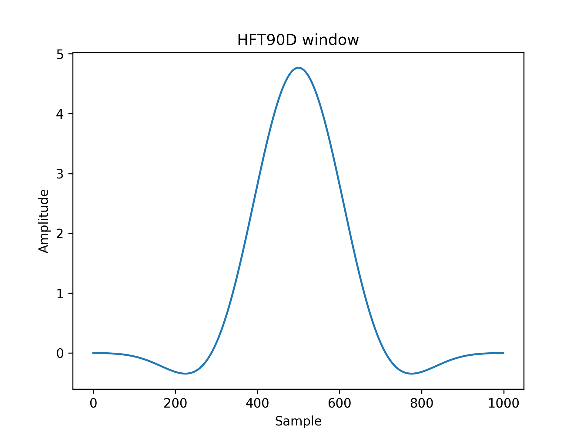
Heinzel describes a flat-top window named "HFT90D" with formula: [2]_ .. math:: w_j = 1 - 1.942604 \cos(z) + 1.340318 \cos(2z) - 0.440811 \cos(3z) + 0.043097 \cos(4z) where .. math:: z = \frac{2 \pi j}{N}, j = 0...N - 1 Since this uses the convention of starting at the origin, to reproduce the window, we need to convert every other coefficient to a positive number:

HFT90D = [1, 1.942604, 1.340318, 0.440811, 0.043097]

✓

The paper states that the highest sidelobe is at -90.2 dB. Reproduce Figure 42 by plotting the window and its frequency response, and confirm the sidelobe level in red:

import numpy as np
from scipy.signal.windows import general_cosine
from scipy.fft import fft, fftshift
import matplotlib.pyplot as plt

✓

window = general_cosine(1000, HFT90D, sym=False)

✓

plt.plot(window)
plt.title("HFT90D window")
plt.ylabel("Amplitude")
plt.xlabel("Sample")

✗

plt.figure()

✗

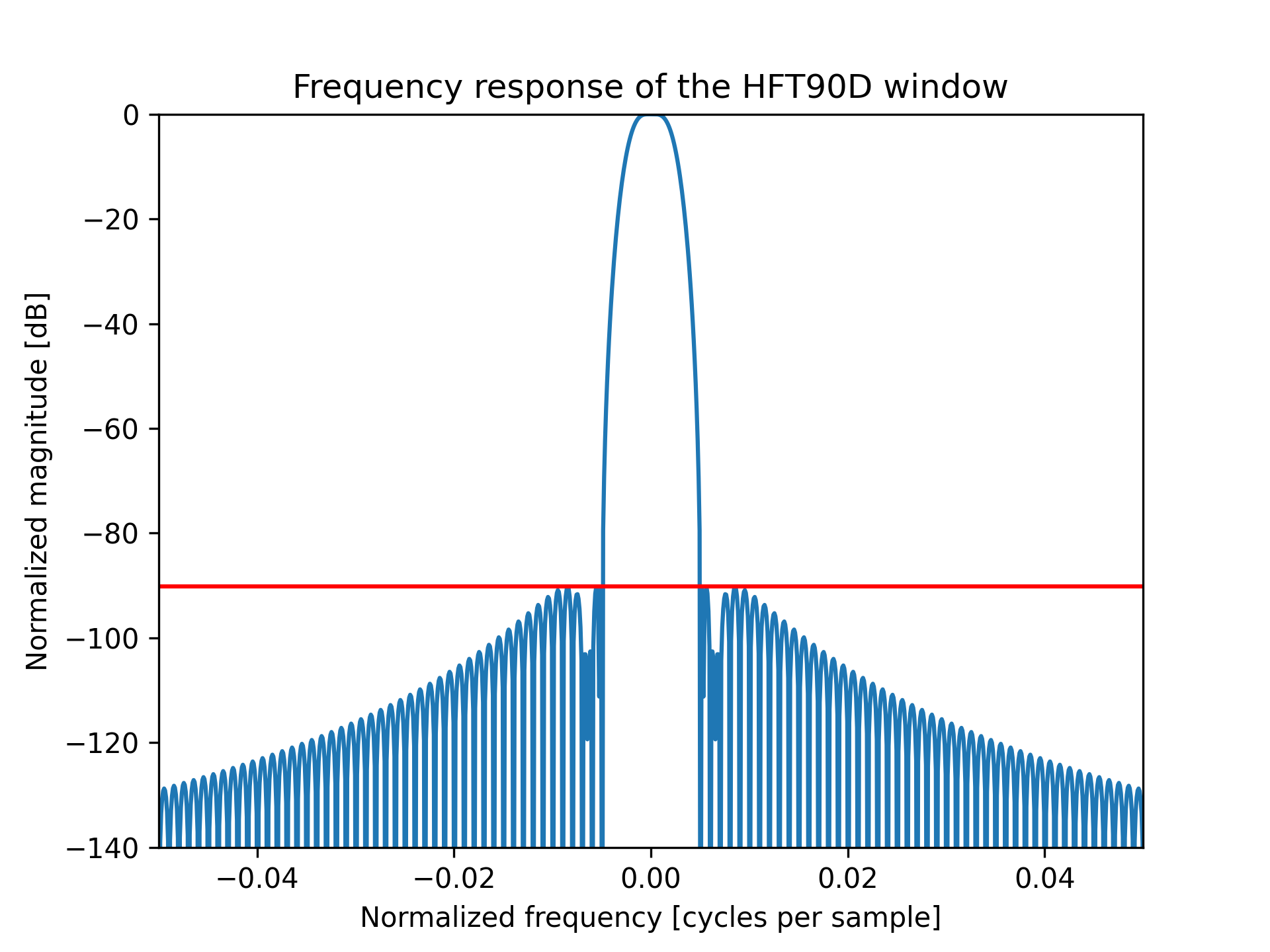
A = fft(window, 10000) / (len(window)/2.0)
freq = np.linspace(-0.5, 0.5, len(A))
response = np.abs(fftshift(A / abs(A).max()))
response = 20 * np.log10(np.maximum(response, 1e-10))

✓

plt.plot(freq, response)
plt.axis([-50/1000, 50/1000, -140, 0])
plt.title("Frequency response of the HFT90D window")
plt.ylabel("Normalized magnitude [dB]")
plt.xlabel("Normalized frequency [cycles per sample]")
plt.axhline(-90.2, color='red')

✗

plt.show()

✓