bundles / scipy latest / scipy / spatial / _geometric_slerp / geometric_slerp
function
scipy.spatial._geometric_slerp:geometric_slerp
Signature
def geometric_slerp ( start : npt.ArrayLike , end : npt.ArrayLike , t : npt.ArrayLike , tol : float = 1e-07 ) → np.ndarray Summary
Geometric spherical linear interpolation.
Extended Summary
The interpolation occurs along a unit-radius great circle arc in arbitrary dimensional space.
Parameters
start: (n_dimensions, ) array-likeSingle n-dimensional input coordinate in a 1-D array-like object.
nmust be greater than 1.end: (n_dimensions, ) array-likeSingle n-dimensional input coordinate in a 1-D array-like object.
nmust be greater than 1.t: float or (n_points,) 1D array-likeA float or 1D array-like of doubles representing interpolation parameters. A common approach is to generate the array with
np.linspace(0, 1, n_pts)for linearly spaced points. Ascending, descending, and scrambled orders are permitted.tol: floatThe absolute tolerance for determining if the start and end coordinates are antipodes.
Returns
result: (t.size, D)An array of doubles containing the interpolated spherical path and including start and end when 0 and 1 t are used. The interpolated values should correspond to the same sort order provided in the t array. The result may be 1-dimensional if
tis a float.
Raises
: ValueErrorIf
startorendare not on the unit n-sphere, or for a variety of degenerate conditions.
Notes
The implementation is based on the mathematical formula provided in [1], and the first known presentation of this algorithm, derived from study of 4-D geometry, is credited to Glenn Davis in a footnote of the original quaternion Slerp publication by Ken Shoemake [2].
Examples
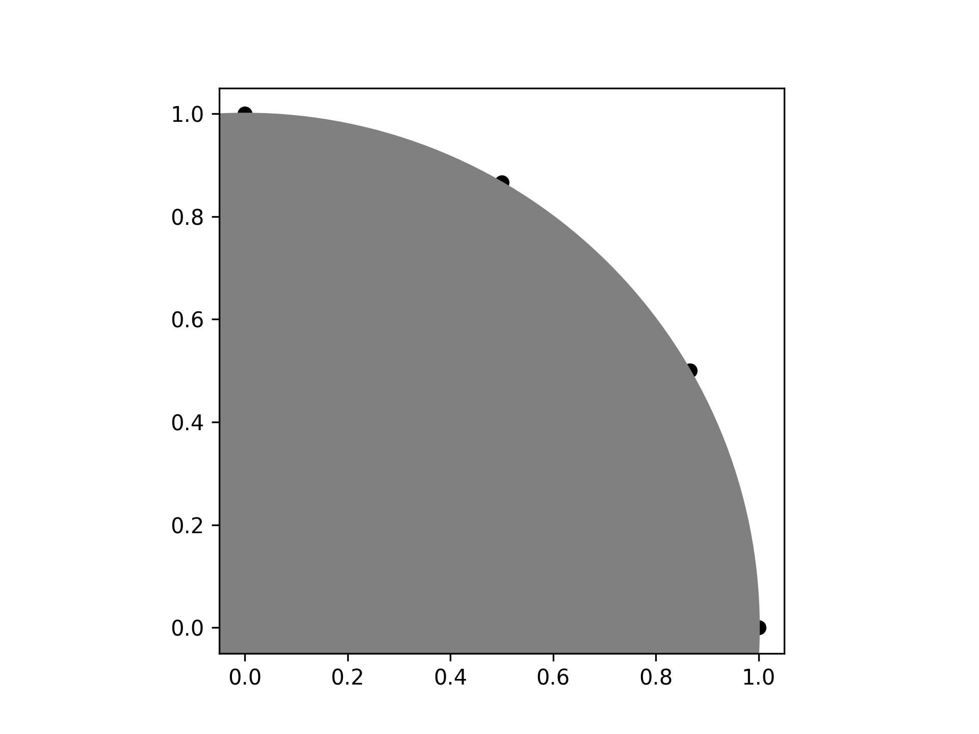
Interpolate four linearly-spaced values on the circumference of a circle spanning 90 degrees:import numpy as np from scipy.spatial import geometric_slerp import matplotlib.pyplot as plt fig = plt.figure() ax = fig.add_subplot(111) start = np.array([1, 0]) end = np.array([0, 1]) t_vals = np.linspace(0, 1, 4) result = geometric_slerp(start, end, t_vals)✓
ax.scatter(result[...,0], result[...,1], c='k')
✗circle = plt.Circle((0, 0), 1, color='grey')
✓ax.add_artist(circle)
✗ax.set_aspect('equal') plt.show()✓
import warnings
opposite_pole = np.array([-1, 0])
✓
with warnings.catch_warnings():
    warnings.simplefilter("ignore", UserWarning)
    geometric_slerp(start,
                    opposite_pole,
                    t_vals)
✗
from mpl_toolkits.mplot3d import proj3d
fig = plt.figure()
ax = fig.add_subplot(111, projection='3d')
✓
u = np.linspace(0, 2 * np.pi, 100)
v = np.linspace(0, np.pi, 100)
x = np.outer(np.cos(u), np.sin(v))
y = np.outer(np.sin(u), np.sin(v))
z = np.outer(np.ones(np.size(u)), np.cos(v))
✓
ax.plot_surface(x, y, z, color='y', alpha=0.1)
✗start = np.array([1, 0, 0]) end = np.array([0, 0, 1]) t_vals = np.linspace(0, 1, 200) result = geometric_slerp(start, end, t_vals)✓
ax.plot(result[...,0],
        result[...,1],
        result[...,2],
        c='k')
✗
plt.show()
✓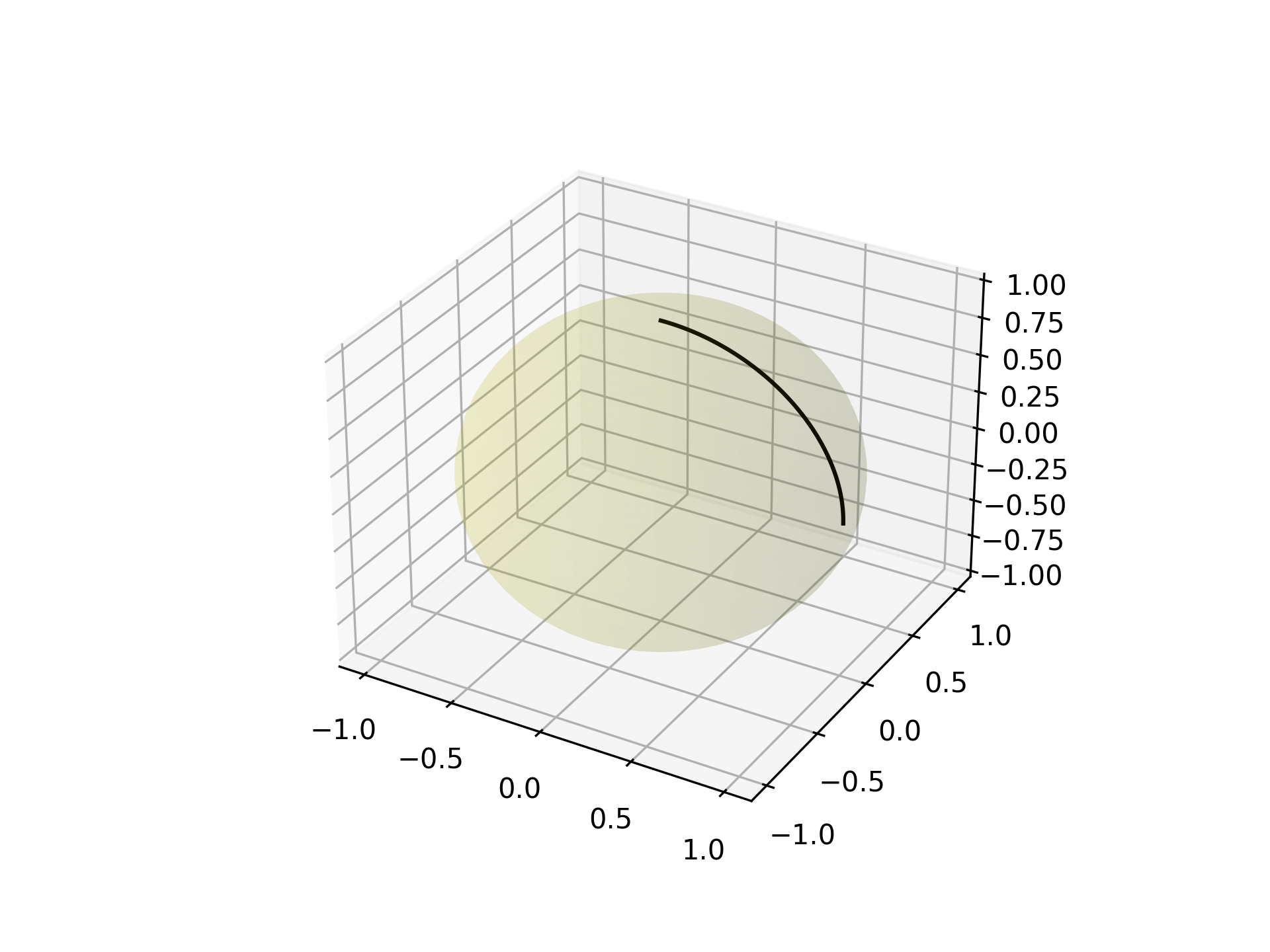
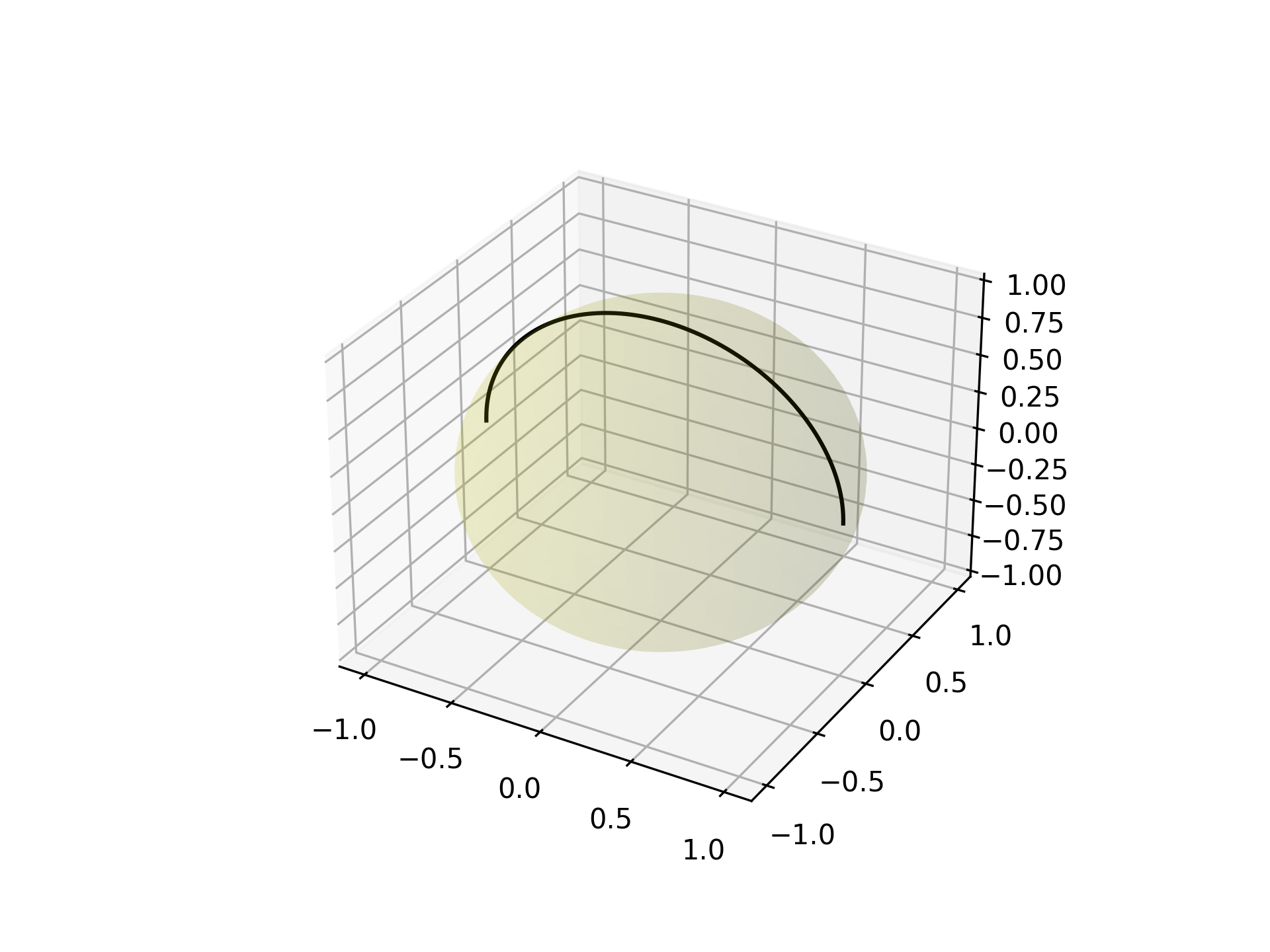
fig = plt.figure()
ax = fig.add_subplot(111, projection='3d')
✓
ax.plot_surface(x, y, z, color='y', alpha=0.1)
✗start = np.array([1, 0, 0]) end = np.array([0, 0, 1]) t_vals = np.linspace(0, 2, 400) result = geometric_slerp(start, end, t_vals)✓
ax.plot(result[...,0], result[...,1], result[...,2], c='k')
✗plt.show()
✓
See also
- scipy.spatial.transform.Slerp
3-D Slerp that works with quaternions
Aliases
-
scipy.spatial.geometric_slerp