`scipy.spatial._spherical_voronoi:SphericalVoronoi`

source: build-install/usr/lib/python3.14/site-packages/scipy/spatial/_spherical_voronoi.py:37

Signature

class SphericalVoronoi(points, radius = 1, center = None, threshold = 1e-06)

Members

Summary

Voronoi diagrams on the surface of a sphere.

Extended Summary

Parameters

points : ndarray of floats, shape (npoints, ndim): Coordinates of points from which to construct a spherical Voronoi diagram.
radius : float, optional: Radius of the sphere (Default: 1)
center : ndarray of floats, shape (ndim,): Center of sphere (Default: origin)
threshold : float: Threshold for detecting duplicate points and mismatches between points and sphere parameters. (Default: 1e-06)

Attributes

points : double array of shape (npoints, ndim): the points in ndim dimensions to generate the Voronoi diagram from
radius : double: radius of the sphere
center : double array of shape (ndim,): center of the sphere
vertices : double array of shape (nvertices, ndim): Voronoi vertices corresponding to points
regions : list of list of integers of shape (npoints, _ ): the n-th entry is a list consisting of the indices of the vertices belonging to the n-th point in points

Methods

calculate_areas: Calculates the areas of the Voronoi regions. For 2D point sets, the regions are circular arcs. The sum of the areas is 2 * pi * radius. For 3D point sets, the regions are spherical polygons. The sum of the areas is 4 * pi * radius**2.

Raises

: ValueError: If there are duplicates in points. If the provided radius is not consistent with points.

Notes

The spherical Voronoi diagram algorithm proceeds as follows. The Convex Hull of the input points (generators) is calculated, and is equivalent to their Delaunay triangulation on the surface of the sphere [Caroli]. The Convex Hull neighbour information is then used to order the Voronoi region vertices around each generator. The latter approach is substantially less sensitive to floating point issues than angle-based methods of Voronoi region vertex sorting.

Empirical assessment of spherical Voronoi algorithm performance suggests quadratic time complexity (loglinear is optimal, but algorithms are more challenging to implement).

Examples

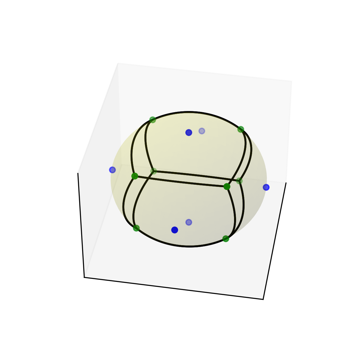
Do some imports and take some points on a cube:

import numpy as np
import matplotlib.pyplot as plt
from scipy.spatial import SphericalVoronoi, geometric_slerp
from mpl_toolkits.mplot3d import proj3d
points = np.array([[0, 0, 1], [0, 0, -1], [1, 0, 0],
                   [0, 1, 0], [0, -1, 0], [-1, 0, 0], ])

✓

Calculate the spherical Voronoi diagram:

radius = 1
center = np.array([0, 0, 0])
sv = SphericalVoronoi(points, radius, center)

✓

Generate plot:

sv.sort_vertices_of_regions()
t_vals = np.linspace(0, 1, 2000)
fig = plt.figure()
ax = fig.add_subplot(111, projection='3d')
u = np.linspace(0, 2 * np.pi, 100)
v = np.linspace(0, np.pi, 100)
x = np.outer(np.cos(u), np.sin(v))
y = np.outer(np.sin(u), np.sin(v))
z = np.outer(np.ones(np.size(u)), np.cos(v))

✓

ax.plot_surface(x, y, z, color='y', alpha=0.1)
ax.scatter(points[:, 0], points[:, 1], points[:, 2], c='b')
ax.scatter(sv.vertices[:, 0], sv.vertices[:, 1], sv.vertices[:, 2],
                   c='g')
for region in sv.regions:
   n = len(region)
   for i in range(n):
       start = sv.vertices[region][i]
       end = sv.vertices[region][(i + 1) % n]
       result = geometric_slerp(start, end, t_vals)
       ax.plot(result[..., 0],
               result[..., 1],
               result[..., 2],
               c='k')

✗

[<mpl_toolkits.mplot3d.art3d.Line3D object at 0x7f3f68208ad0>]
[<mpl_toolkits.mplot3d.art3d.Line3D object at 0x7f3f6820acf0>]
[<mpl_toolkits.mplot3d.art3d.Line3D object at 0x7f3f682081a0>]
[<mpl_toolkits.mplot3d.art3d.Line3D object at 0x7f3f68208ec0>]
[<mpl_toolkits.mplot3d.art3d.Line3D object at 0x7f3f6820a660>]
[<mpl_toolkits.mplot3d.art3d.Line3D object at 0x7f3f68209a90>]
[<mpl_toolkits.mplot3d.art3d.Line3D object at 0x7f3f68209010>]
[<mpl_toolkits.mplot3d.art3d.Line3D object at 0x7f3f6820be00>]
[<mpl_toolkits.mplot3d.art3d.Line3D object at 0x7f3f68208050>]
[<mpl_toolkits.mplot3d.art3d.Line3D object at 0x7f3f68208d70>]
[<mpl_toolkits.mplot3d.art3d.Line3D object at 0x7f3f682092b0>]
[<mpl_toolkits.mplot3d.art3d.Line3D object at 0x7f3f6820bcb0>]
[<mpl_toolkits.mplot3d.art3d.Line3D object at 0x7f3f6820aba0>]
[<mpl_toolkits.mplot3d.art3d.Line3D object at 0x7f3f682082f0>]
[<mpl_toolkits.mplot3d.art3d.Line3D object at 0x7f3f6820b4d0>]
[<mpl_toolkits.mplot3d.art3d.Line3D object at 0x7f3f68209e80>]
[<mpl_toolkits.mplot3d.art3d.Line3D object at 0x7f3f6820ae40>]
[<mpl_toolkits.mplot3d.art3d.Line3D object at 0x7f3f68209400>]
[<mpl_toolkits.mplot3d.art3d.Line3D object at 0x7f3f68209160>]
[<mpl_toolkits.mplot3d.art3d.Line3D object at 0x7f3f682097f0>]
[<mpl_toolkits.mplot3d.art3d.Line3D object at 0x7f3f6820ba10>]
[<mpl_toolkits.mplot3d.art3d.Line3D object at 0x7f3f68209d30>]
[<mpl_toolkits.mplot3d.art3d.Line3D object at 0x7f3f687d9be0>]
[<mpl_toolkits.mplot3d.art3d.Line3D object at 0x7f3f687d9550>]

ax.azim = 10
ax.elev = 40
_ = ax.set_xticks([])
_ = ax.set_yticks([])
_ = ax.set_zticks([])
fig.set_size_inches(4, 4)
plt.show()

✓

Aliases

scipy.spatial.SphericalVoronoi