bundles / scipy 1.17.1 / scipy / signal / _ltisys / dbode
function
scipy.signal._ltisys:dbode
source: /scipy/signal/_ltisys.py :3455
Signature
def dbode ( system , w = None , n = 100 ) Summary
Calculate Bode magnitude and phase data of a discrete-time system.
Parameters
system: dlti | tupleAn instance of the LTI class dlti or a tuple describing the system. The number of elements in the tuple determine the interpretation. I.e.:
system: Instance of LTI class dlti. Note that derived instances, such as instances of TransferFunction, ZerosPolesGain, or StateSpace, are allowed as well.(num, den, dt): Rational polynomial as described in TransferFunction. The coefficients of the polynomials should be specified in descending exponent order, e.g., z² + 3z + 5 would be represented as[1, 3, 5].(zeros, poles, gain, dt): Zeros, poles, gain form as described in ZerosPolesGain.(A, B, C, D, dt): State-space form as described in StateSpace.
w: array_like, optionalArray of frequencies normalized to the Nyquist frequency being π, i.e., having unit radiant / sample. Magnitude and phase data is calculated for every value in this array. If not given, a reasonable set will be calculated.
n: int, optionalNumber of frequency points to compute if
wis not given. Thenfrequencies are logarithmically spaced in an interval chosen to include the influence of the poles and zeros of the system.
Returns
w: 1D ndarrayArray of frequencies normalized to the Nyquist frequency being
np.pi/dtwithdtbeing the sampling interval of thesystemparameter. The unit is rad/s assumingdtis in seconds.mag: 1D ndarrayMagnitude array in dB
phase: 1D ndarrayPhase array in degrees
Notes
This function is a convenience wrapper around dfreqresp for extracting magnitude and phase from the calculated complex-valued amplitude of the frequency response.
Array API Standard Support
dbode has experimental support for Python Array API Standard compatible backends in addition to NumPy. Please consider testing these features by setting an environment variable SCIPY_ARRAY_API=1 and providing CuPy, PyTorch, JAX, or Dask arrays as array arguments. The following combinations of backend and device (or other capability) are supported.
====================  ====================  ====================
Library               CPU                   GPU
====================  ====================  ====================
NumPy                 ✅                     n/a
CuPy                  n/a                   ⛔
PyTorch               ⛔                     ⛔
JAX                   ⛔                     ⛔
Dask                  ⛔                     n/a
====================  ====================  ====================
See
dev-arrayapifor more information.
Examples
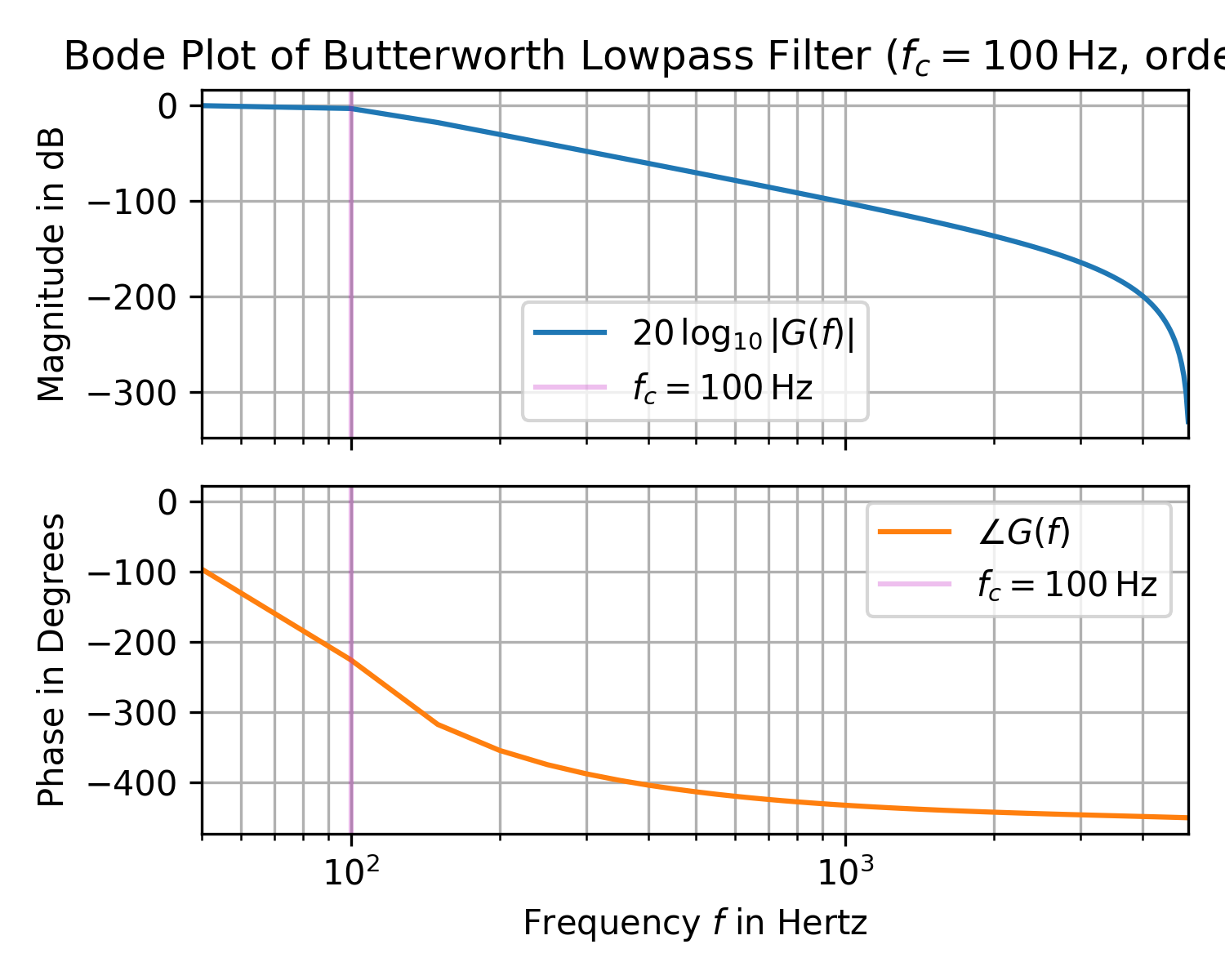
The following example shows how to create a Bode plot of a 5-th order Butterworth lowpass filter with a corner frequency of 100 Hz:import matplotlib.pyplot as plt import numpy as np from scipy import signal T = 1e-4 # sampling interval in s f_c, o = 1e2, 5 # corner frequency in Hz (i.e., -3 dB value) and filter order bb, aa = signal.butter(o, f_c, 'lowpass', fs=1/T) w, mag, phase = signal.dbode((bb, aa, T)) w /= 2*np.pi # convert unit of frequency into Hertz fg, (ax0, ax1) = plt.subplots(2, 1, sharex='all', figsize=(5, 4), tight_layout=True)✓
ax0.set_title("Bode Plot of Butterworth Lowpass Filter " +
              rf"($f_c={f_c:g}\,$Hz, order={o})")
ax0.set_ylabel(r"Magnitude in dB")
ax1.set(ylabel=r"Phase in Degrees",
        xlabel="Frequency $f$ in Hertz", xlim=(w[1], w[-1]))
ax0.semilogx(w, mag, 'C0-', label=r"$20\,\log_{10}|G(f)|$")  # Magnitude plot
ax1.semilogx(w, phase, 'C1-', label=r"$\angle G(f)$")  # Phase plot
for ax_ in (ax0, ax1):
    ax_.axvline(f_c, color='m', alpha=0.25, label=rf"${f_c=:g}\,$Hz")
    ax_.grid(which='both', axis='x')  # plot major & minor vertical grid lines
    ax_.grid(which='major', axis='y')
    ax_.legend()
✗
plt.show()
✓
See also
Aliases
-
scipy.signal.dbode