{ } Raw JSON

bundles / scipy 1.17.1 / scipy / signal / _ltisys / lsim

function

`scipy.signal._ltisys:lsim`

source: /scipy/signal/_ltisys.py :1765

Signature

def lsim ( system , U , T , X0 = None , interp = True )

Summary

Simulate output of a continuous-time linear system.

Parameters

system : an instance of the LTI class or a tuple describing the system.

The following gives the number of elements in the tuple and the interpretation:

1: (instance of lti)
2: (num, den)
3: (zeros, poles, gain)
4: (A, B, C, D)

U : array_like

An input array describing the input at each time T (interpolation is assumed between given times). If there are multiple inputs, then each column of the rank-2 array represents an input. If U = 0 or None, a zero input is used.

T : array_like

The time steps at which the input is defined and at which the output is desired. Must be nonnegative, increasing, and equally spaced.

X0 : array_like, optional

The initial conditions on the state vector (zero by default).

interp : bool, optional

Whether to use linear (True, the default) or zero-order-hold (False) interpolation for the input array.

Returns

T : 1D ndarray: Time values for the output.
yout : 1D ndarray: System response.
xout : ndarray: Time evolution of the state vector.

Notes

If (num, den) is passed in for system, coefficients for both the numerator and denominator should be specified in descending exponent order (e.g. s^2 + 3s + 5 would be represented as [1, 3, 5]).

Array API Standard Support

lsim has experimental support for Python Array API Standard compatible backends in addition to NumPy. Please consider testing these features by setting an environment variable SCIPY_ARRAY_API=1 and providing CuPy, PyTorch, JAX, or Dask arrays as array arguments. The following combinations of backend and device (or other capability) are supported.

====================  ====================  ====================
Library               CPU                   GPU
====================  ====================  ====================
NumPy                 ✅                     n/a                 
CuPy                  n/a                   ⛔                   
PyTorch               ⛔                     ⛔                   
JAX                   ⛔                     ⛔                   
Dask                  ⛔                     n/a                 
====================  ====================  ====================

See dev-arrayapi for more information.

Examples

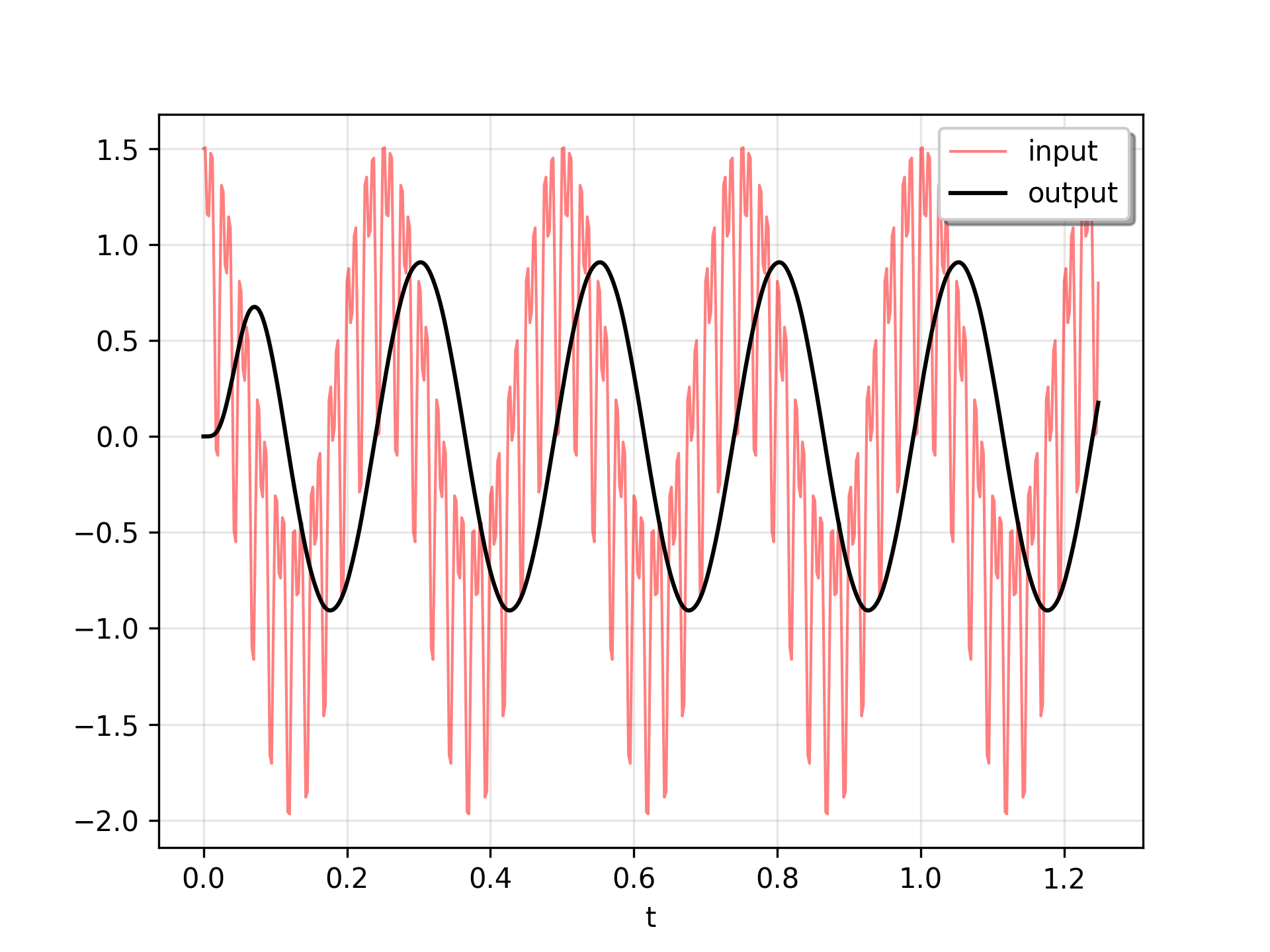
We'll use `lsim` to simulate an analog Bessel filter applied to a signal.

import numpy as np
from scipy.signal import bessel, lsim
import matplotlib.pyplot as plt

✓

Create a low-pass Bessel filter with a cutoff of 12 Hz.

b, a = bessel(N=5, Wn=2*np.pi*12, btype='lowpass', analog=True)

✓

Generate data to which the filter is applied.

t = np.linspace(0, 1.25, 500, endpoint=False)

✓

The input signal is the sum of three sinusoidal curves, with frequencies 4 Hz, 40 Hz, and 80 Hz. The filter should mostly eliminate the 40 Hz and 80 Hz components, leaving just the 4 Hz signal.

u = (np.cos(2*np.pi*4*t) + 0.6*np.sin(2*np.pi*40*t) +
     0.5*np.cos(2*np.pi*80*t))

✓

Simulate the filter with `lsim`.

tout, yout, xout = lsim((b, a), U=u, T=t)

✓

Plot the result.

plt.plot(t, u, 'r', alpha=0.5, linewidth=1, label='input')
plt.plot(tout, yout, 'k', linewidth=1.5, label='output')
plt.legend(loc='best', shadow=True, framealpha=1)

✗

plt.grid(alpha=0.3)

✓

plt.xlabel('t')

✗

plt.show()

✓

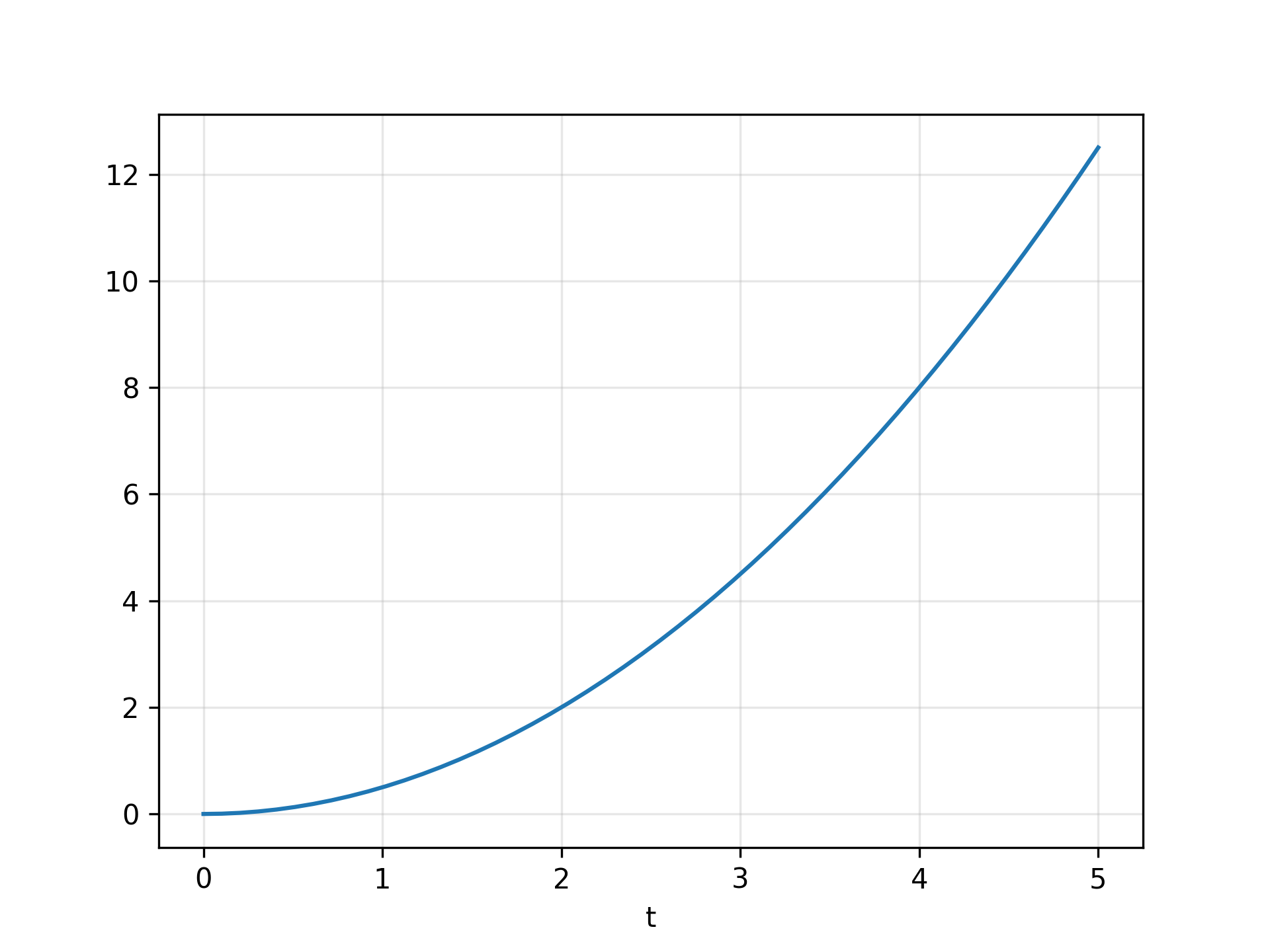
In a second example, we simulate a double integrator ``y'' = u``, with a constant input ``u = 1``. We'll use the state space representation of the integrator.

from scipy.signal import lti
A = np.array([[0.0, 1.0], [0.0, 0.0]])
B = np.array([[0.0], [1.0]])
C = np.array([[1.0, 0.0]])
D = 0.0
system = lti(A, B, C, D)

✓

`t` and `u` define the time and input signal for the system to be simulated.

t = np.linspace(0, 5, num=50)
u = np.ones_like(t)

✓

Compute the simulation, and then plot `y`. As expected, the plot shows the curve ``y = 0.5*t**2``.

tout, y, x = lsim(system, u, t)

✓

plt.plot(t, y)

✗

plt.grid(alpha=0.3)

✓

plt.xlabel('t')

✗

plt.show()

✓

Aliases

scipy.signal.lsim