`scipy.signal._ltisys:dstep`

source: /scipy/signal/_ltisys.py :3253

Signature

def dstep ( system , x0 = None , t = None , n = None )

Summary

Step response of discrete-time system.

Parameters

system : dlti | tuple

An instance of the LTI class dlti or a tuple describing the system. The number of elements in the tuple determine the interpretation. I.e.:

system: Instance of LTI class dlti. Note that derived instances, such as instances of TransferFunction, ZerosPolesGain, or StateSpace, are allowed as well.
(num, den, dt): Rational polynomial as described in TransferFunction. The coefficients of the polynomials should be specified in descending exponent order, e.g., z² + 3z + 5 would be represented as [1, 3, 5].
(zeros, poles, gain, dt): Zeros, poles, gain form as described in ZerosPolesGain.
(A, B, C, D, dt): State-space form as described in StateSpace.

x0 : array_like, optional

Initial state-vector. Defaults to zero.

t : array_like, optional

Time points. Computed if not given.

n : int, optional

The number of time points to compute (if t is not given).

Returns

tout : ndarray: Output time points, as a 1-D array.
yout : tuple of ndarray: Step response of system. Each element of the tuple represents the output of the system based on a step response to each input.

Notes

Array API Standard Support

dstep has experimental support for Python Array API Standard compatible backends in addition to NumPy. Please consider testing these features by setting an environment variable SCIPY_ARRAY_API=1 and providing CuPy, PyTorch, JAX, or Dask arrays as array arguments. The following combinations of backend and device (or other capability) are supported.

====================  ====================  ====================
Library               CPU                   GPU
====================  ====================  ====================
NumPy                 ✅                     n/a                 
CuPy                  n/a                   ⛔                   
PyTorch               ⛔                     ⛔                   
JAX                   ⛔                     ⛔                   
Dask                  ⛔                     n/a                 
====================  ====================  ====================

See dev-arrayapi for more information.

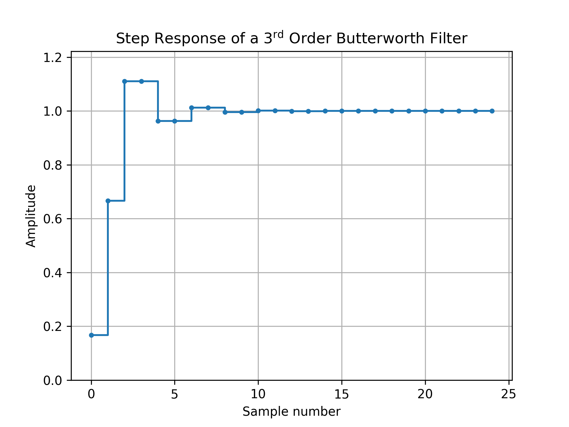
Examples

The following example illustrates how to create a digital Butterworth filer and plot its step response:

import numpy as np
from scipy import signal
import matplotlib.pyplot as plt
dt = 1  # sampling interval is one => time unit is sample number
bb, aa = signal.butter(3, 0.25, fs=1/dt)
t, y = signal.dstep((bb, aa, dt), n=25)
fig0, ax0 = plt.subplots()

✓

ax0.step(t, np.squeeze(y), '.-', where='post')
ax0.set_title(r"Step Response of a $3^\text{rd}$ Order Butterworth Filter")
ax0.set(xlabel='Sample number', ylabel='Amplitude', ylim=(0, 1.1*np.max(y)))

✗

ax0.grid()
plt.show()

✓

Aliases

scipy.signal.dstep