bundles / scipy 1.17.1 / scipy / signal / _short_time_fft / ShortTimeFFT / from_dual
classmethod
scipy.signal._short_time_fft:ShortTimeFFT.from_dual
Summary
Instantiate a ShortTimeFFT by only providing a dual window.
Extended Summary
If an STFT is invertible, it is possible to calculate the window win from a given dual window dual_win. All other parameters have the same meaning as in the initializer of ShortTimeFFT.
As explained in the tutorial_stft section of the user_guide, an invertible STFT can be interpreted as series expansion of time-shifted and frequency modulated dual windows. E.g., the series coefficient S[q,p] belongs to the term, which shifted dual_win by p * delta_t and multiplied it by exp( 2 * j * pi * t * q * delta_f).
Examples
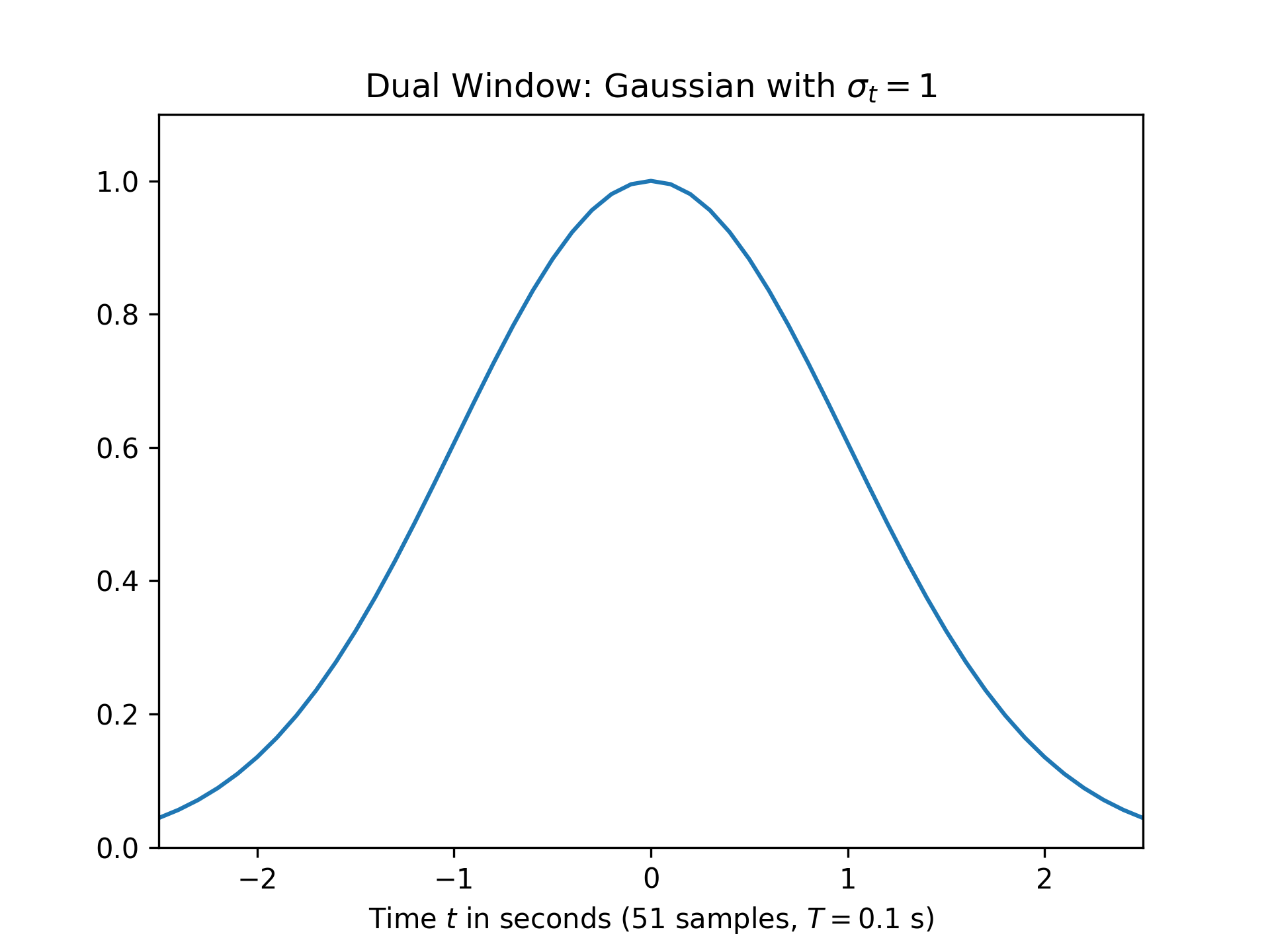
The following example discusses decomposing a signal into time- and frequency-shifted Gaussians. A Gaussian with standard deviation of one made up of 51 samples will be used:import numpy as np import matplotlib.pyplot as plt from scipy.signal import ShortTimeFFT from scipy.signal.windows import gaussian T, N = 0.1, 51 d_win = gaussian(N, std=1/T, sym=True) # symmetric Gaussian window t = T * (np.arange(N) - N//2) fg1, ax1 = plt.subplots()✓
ax1.set_title(r"Dual Window: Gaussian with $\sigma_t=1$")
ax1.set(xlabel=f"Time $t$ in seconds ({N} samples, $T={T}$ s)",
       xlim=(t[0], t[-1]), ylim=(0, 1.1*np.max(d_win)))
ax1.plot(t, d_win, 'C0-')
✗
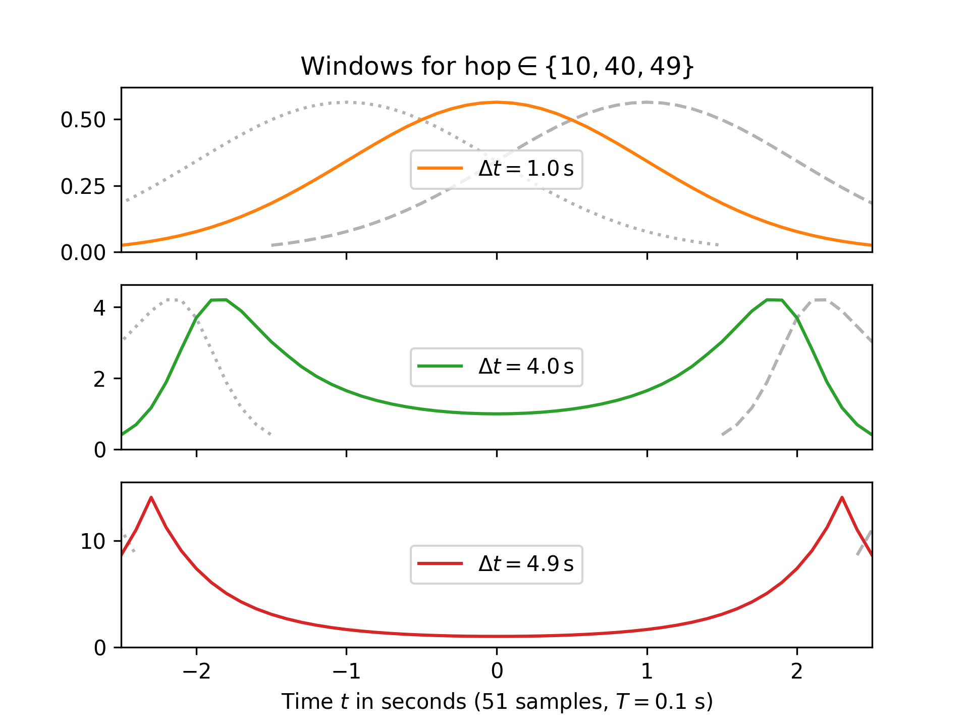
fig2, axx = plt.subplots(3, 1, sharex='all')
✓axx[0].set_title(r"Windows for hop$\in\{10, 40, 49\}$") for c_, h_ in enumerate([10, 40, 49]): SFT = ShortTimeFFT.from_dual(d_win, h_, 1/T) axx[c_].plot(t + h_ * T, SFT.win, 'k--', alpha=.3, label=None) axx[c_].plot(t - h_ * T, SFT.win, 'k:', alpha=.3, label=None) axx[c_].plot(t, SFT.win, f'C{c_+1}', label=r"$\Delta t=%0.1f\,$s" % SFT.delta_t) axx[c_].set_ylim(0, 1.1*max(SFT.win)) axx[c_].legend(loc='center') axx[-1].set(xlabel=f"Time $t$ in seconds ({N} samples, $T={T}$ s)", xlim=(t[0], t[-1]))✗
plt.show()
✓
See also
- ShortTimeFFT
Create instance using standard initializer.
- from_window
Create instance by wrapping
get_window.
Aliases
-
scipy.signal.ShortTimeFFT.from_dual