bundles / scipy 1.17.1 / scipy / signal / _short_time_fft / ShortTimeFFT
class
scipy.signal._short_time_fft:ShortTimeFFT
Signature
class ShortTimeFFT ( win : np.ndarray , hop : int , fs : float , * , fft_mode : FFT_MODE_TYPE = onesided , mfft : int | None = None , dual_win : np.ndarray | None = None , scale_to : Literal['magnitude', 'psd'] | None = None , phase_shift : int | None = 0 ) Members
-
__annotate__ -
__init__ -
_fft_func -
_ifft_func -
_post_padding -
_x_slices -
extent -
from_dual -
from_win_equals_dual -
from_window -
istft -
k_max -
nearest_k_p -
p_max -
p_num -
p_range -
scale_to -
spectrogram -
stft -
stft_detrend -
t -
upper_border_begin
Summary
Provide a parametrized discrete Short-time Fourier transform (stft) and its inverse (istft).
Extended Summary
The ~ShortTimeFFT.stft calculates sequential FFTs by sliding a window (win) over an input signal by hop increments. It can be used to quantify the change of the spectrum over time.
The ~ShortTimeFFT.stft is represented by a complex-valued matrix S[q,p] where the p-th column represents an FFT with the window centered at the time t[p] = p * delta_t = p * hop * T where T is the sampling interval of the input signal. The q-th row represents the values at the frequency f[q] = q * delta_f with delta_f = 1 / (mfft * T) being the bin width of the FFT.
The inverse STFT ~ShortTimeFFT.istft is calculated by reversing the steps of the STFT: Take the IFFT of the p-th slice of S[q,p] and multiply the result with the so-called dual window (see dual_win). Shift the result by p * delta_t and add the result to previous shifted results to reconstruct the signal. If only the dual window is known and the STFT is invertible, from_dual can be used to instantiate this class.
By default, the so-called canonical dual window is used. It is the window with minimal energy among all possible dual windows. from_win_equals_dual and closest_STFT_dual_window provide means for utilizing alterantive dual windows. Note that win is also always a dual window of dual_win.
Due to the convention of time t = 0 being at the first sample of the input signal, the STFT values typically have negative time slots. Hence, negative indexes like p_min or k_min do not indicate counting backwards from an array's end like in standard Python indexing but being left of t = 0.
More detailed information can be found in the tutorial_stft section of the user_guide.
Note that all parameters of the initializer, except scale_to (which uses scaling) have identical named attributes.
Parameters
win: np.ndarrayThe window must be a real- or complex-valued 1d array.
hop: intThe increment in samples, by which the window is shifted in each step.
fs: floatSampling frequency of input signal and window. Its relation to the sampling interval
TisT = 1 / fs.fft_mode: 'twosided', 'centered', 'onesided', 'onesided2X'Mode of FFT to be used (default 'onesided'). See property
fft_modefor details.mfft: int | NoneLength of the FFT used, if a zero padded FFT is desired. If
None(default), the length of the windowwinis used.dual_win: np.ndarray | NoneThe dual window of
win. If set toNone, it is calculated if needed.scale_to: 'magnitude', 'psd' | NoneIf not
None(default) the window function is scaled, so each STFT column represents either a 'magnitude' or a power spectral density ('psd') spectrum. This parameter sets the propertyscalingto the same value. See methodscale_tofor details.phase_shift: int | NoneIf set, add a linear phase
phase_shift/mfft*fto each frequencyf. The default value of 0 ensures that there is no phase shift on the zeroth slice (in which t=0 is centered). See propertyphase_shiftfor more details.
Notes
A typical STFT application is the creation of various types of time-frequency plots, often subsumed under the term "spectrogram". Note that this term is also used to explecitly refer to the absolute square of a STFT [11], as done in spectrogram.
The STFT can also be used for filtering and filter banks as discussed in [12].
Array API Standard Support
ShortTimeFFT has experimental support for Python Array API Standard compatible backends in addition to NumPy. Please consider testing these features by setting an environment variable SCIPY_ARRAY_API=1 and providing CuPy, PyTorch, JAX, or Dask arrays as array arguments. The following combinations of backend and device (or other capability) are supported.
====================  ====================  ====================
Library               CPU                   GPU
====================  ====================  ====================
NumPy                 ✅                     n/a
CuPy                  n/a                   ⛔
PyTorch               ⛔                     ⛔
JAX                   ⛔                     ⛔
Dask                  ⛔                     n/a
====================  ====================  ====================
See
dev-arrayapifor more information.
Examples
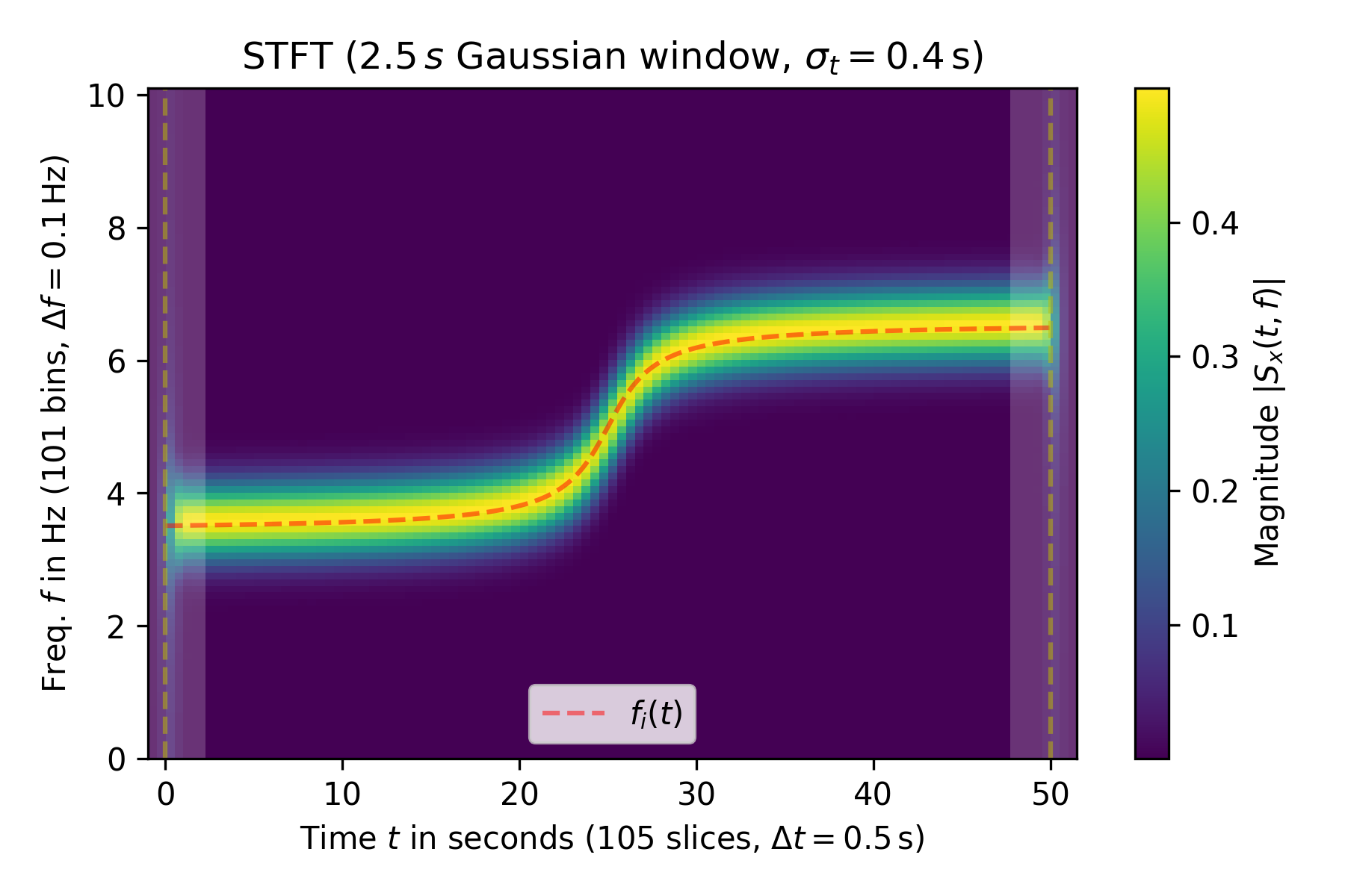
The following example shows the magnitude of the STFT of a sine with varying frequency :math:`f_i(t)` (marked by a red dashed line in the plot):import numpy as np import matplotlib.pyplot as plt from scipy.signal import ShortTimeFFT from scipy.signal.windows import gaussian T_x, N = 1 / 20, 1000 # 20 Hz sampling rate for 50 s signal t_x = np.arange(N) * T_x # time indexes for signal f_i = 1 * np.arctan((t_x - t_x[N // 2]) / 2) + 5 # varying frequency x = np.sin(2*np.pi*np.cumsum(f_i)*T_x) # the signal✓
g_std = 8  # standard deviation for Gaussian window in samples
w = gaussian(50, std=g_std, sym=True)  # symmetric Gaussian window
SFT = ShortTimeFFT(w, hop=10, fs=1/T_x, mfft=200, scale_to='magnitude')
Sx = SFT.stft(x)  # perform the STFT
✓
fig1, ax1 = plt.subplots(figsize=(6., 4.))  # enlarge plot a bit
t_lo, t_hi = SFT.extent(N)[:2]  # time range of plot
✓
ax1.set_title(rf"STFT ({SFT.m_num*SFT.T:g}$\,s$ Gaussian window, " +
              rf"$\sigma_t={g_std*SFT.T}\,$s)")
ax1.set(xlabel=f"Time $t$ in seconds ({SFT.p_num(N)} slices, " +
               rf"$\Delta t = {SFT.delta_t:g}\,$s)",
        ylabel=f"Freq. $f$ in Hz ({SFT.f_pts} bins, " +
               rf"$\Delta f = {SFT.delta_f:g}\,$Hz)",
        xlim=(t_lo, t_hi))
✗
im1 = ax1.imshow(abs(Sx), origin='lower', aspect='auto',
                 extent=SFT.extent(N), cmap='viridis')
✓
ax1.plot(t_x, f_i, 'r--', alpha=.5, label='$f_i(t)$')
fig1.colorbar(im1, label="Magnitude $|S_x(t, f)|$")
for t0_, t1_ in [(t_lo, SFT.lower_border_end[0] * SFT.T),
                 (SFT.upper_border_begin(N)[0] * SFT.T, t_hi)]:
    ax1.axvspan(t0_, t1_, color='w', linewidth=0, alpha=.2)
for t_ in [0, N * SFT.T]:  # mark signal borders with vertical line:
    ax1.axvline(t_, color='y', linestyle='--', alpha=0.5)
ax1.legend()
✗
fig1.tight_layout()
plt.show()
✓
SFT.invertible  # check if invertible
x1 = SFT.istft(Sx, k1=N)
np.allclose(x, x1)
✓
N2 = SFT.nearest_k_p(N // 2)
Sx0 = SFT.stft(x[:N2])
Sx1 = SFT.stft(x[N2:])
✓
p0_ub = SFT.upper_border_begin(N2)[1] - SFT.p_min
p1_le = SFT.lower_border_end[1] - SFT.p_min
Sx01 = np.hstack((Sx0[:, :p0_ub],
                  Sx0[:, p0_ub:] + Sx1[:, :p1_le],
                  Sx1[:, p1_le:]))
np.allclose(Sx01, Sx)  # Compare with SFT of complete signal
✓
y_p = SFT.istft(Sx, N//3, N//2)
np.allclose(y_p, x[N//3:N//2])
✓
Aliases
-
scipy.signal.ShortTimeFFT