bundles / scipy 1.17.1 / scipy / signal / _waveforms / chirp

function

`scipy.signal._waveforms:chirp`

source: /scipy/signal/_waveforms.py :251

Signature

   def     chirp (    t    ,    f0    ,    t1    ,    f1    ,    method    =  linear   ,    phi    =  0   ,    vertex_zero    =  True   ,  * ,     complex    =  False     )

Summary

Frequency-swept cosine generator.

Extended Summary

In the following, 'Hz' should be interpreted as 'cycles per unit'; there is no requirement here that the unit is one second. The important distinction is that the units of rotation are cycles, not radians. Likewise, t could be a measurement of space instead of time.

Parameters

t : array_like: Times at which to evaluate the waveform.
f0 : float: Frequency (e.g. Hz) at time t=0.
t1 : float: Time at which f1 is specified.
f1 : float: Frequency (e.g. Hz) of the waveform at time t1.
method : {'linear', 'quadratic', 'logarithmic', 'hyperbolic'}, optional: Kind of frequency sweep. If not given, linear is assumed. See Notes below for more details.
phi : float, optional: Phase offset, in degrees. Default is 0.
vertex_zero : bool, optional: This parameter is only used when method is 'quadratic'. It determines whether the vertex of the parabola that is the graph of the frequency is at t=0 or t=t1.
complex : bool, optional: This parameter creates a complex-valued analytic signal instead of a real-valued signal. It allows the use of complex baseband (in communications domain). Default is False.
versionadded 1.15.0

Returns

y : ndarray: A numpy array containing the signal evaluated at t with the requested time-varying frequency. More precisely, the function returns exp(1j*phase + 1j*(pi/180)*phi) if complex else cos(phase + (pi/180)*phi) where phase is the integral (from 0 to t) of 2*pi*f(t). The instantaneous frequency f(t) is defined below.

Notes

There are four possible options for the parameter method, which have a (long) standard form and some allowed abbreviations. The formulas for the instantaneous frequency $f (t)$ of the generated signal are as follows:

Parameter method in ('linear', 'lin', 'li'):
$f (t) = f_{0} + β t with β = \frac{f _{1} - f _{0}}{t _{1}}$
Frequency $f (t)$ varies linearly over time with a constant rate $β$ .
Parameter method in ('quadratic', 'quad', 'q'):
f(t) = \begin{cases} f_0 + \beta\, t^2 & \text{if vertex_zero is True,}\\ f_1 + \beta\, (t_1 - t)^2 & \text{otherwise,} \end{cases} \quad\text{with}\quad \beta = \frac{f_1 - f_0}{t_1^2}
The graph of the frequency f(t) is a parabola through $(0, f_{0})$ and $(t_{1}, f_{1})$ . By default, the vertex of the parabola is at $(0, f_{0})$ . If vertex_zero is False, then the vertex is at $(t_{1}, f_{1})$ . To use a more general quadratic function, or an arbitrary polynomial, use the function scipy.signal.sweep_poly.
Parameter method in ('logarithmic', 'log', 'lo'):
$f (t) = f_{0} (\frac{f _{1}}{f _{0}})^{t / t_{1}}$
$f_{0}$ and $f_{1}$ must be nonzero and have the same sign. This signal is also known as a geometric or exponential chirp.
Parameter method in ('hyperbolic', 'hyp'):
$f (t) = \frac{α}{β t + γ} with α = f_{0} f_{1} t_{1}, β = f_{0} - f_{1}, γ = f_{1} t_{1}$
$f_{0}$ and $f_{1}$ must be nonzero.

Array API Standard Support

chirp has experimental support for Python Array API Standard compatible backends in addition to NumPy. Please consider testing these features by setting an environment variable SCIPY_ARRAY_API=1 and providing CuPy, PyTorch, JAX, or Dask arrays as array arguments. The following combinations of backend and device (or other capability) are supported.

====================  ====================  ====================
Library               CPU                   GPU
====================  ====================  ====================
NumPy                 ✅                     n/a                 
CuPy                  n/a                   ⛔                   
PyTorch               ⛔                     ⛔                   
JAX                   ⛔                     ⛔                   
Dask                  ⛔                     n/a                 
====================  ====================  ====================

See dev-arrayapi for more information.

Examples

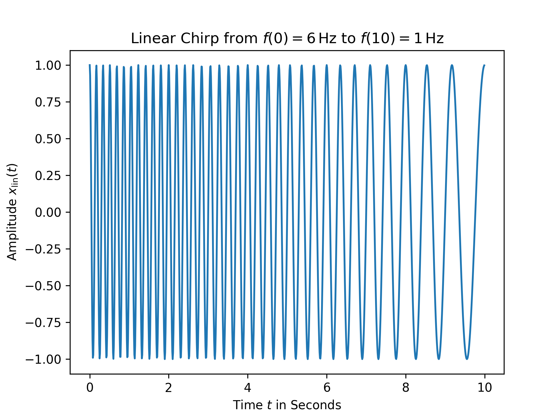
For the first example, a linear chirp ranging from 6 Hz to 1 Hz over 10 seconds is plotted:

import numpy as np
from matplotlib.pyplot import tight_layout
from scipy.signal import chirp, square, ShortTimeFFT
from scipy.signal.windows import gaussian
import matplotlib.pyplot as plt
N, T = 1000, 0.01  # number of samples and sampling interval for 10 s signal
t = np.arange(N) * T  # timestamps
x_lin = chirp(t, f0=6, f1=1, t1=10, method='linear')
fg0, ax0 = plt.subplots()

✓

ax0.set_title(r"Linear Chirp from $f(0)=6\,$Hz to $f(10)=1\,$Hz")
ax0.set(xlabel="Time $t$ in Seconds", ylabel=r"Amplitude $x_\text{lin}(t)$")
ax0.plot(t, x_lin)

✗

plt.show()

✓

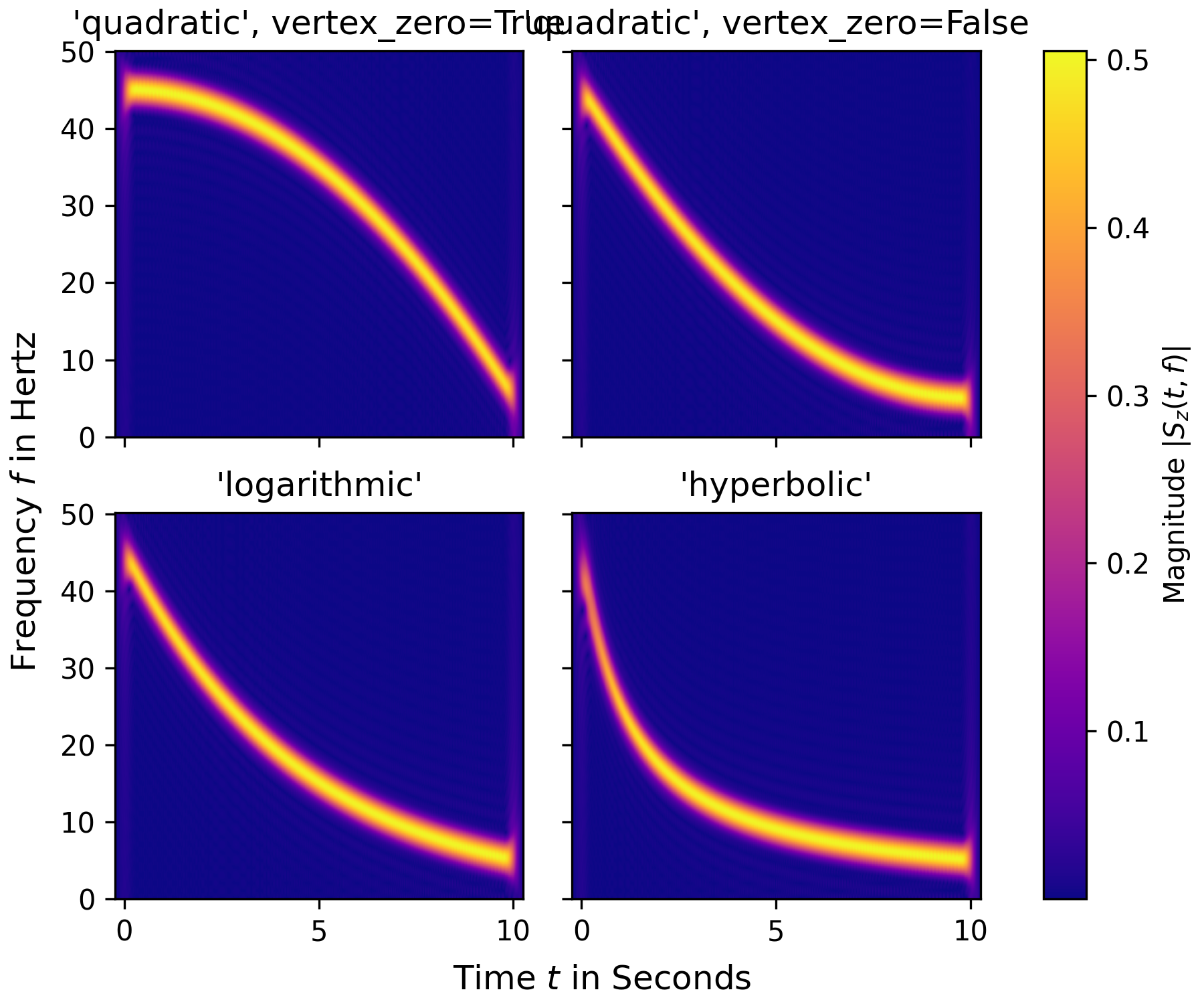
The following four plots each show the short-time Fourier transform of a chirp ranging from 45 Hz to 5 Hz with different values for the parameter `method` (and `vertex_zero`):

x_qu0 = chirp(t, f0=45, f1=5, t1=N*T, method='quadratic', vertex_zero=True)
x_qu1 = chirp(t, f0=45, f1=5, t1=N*T, method='quadratic', vertex_zero=False)
x_log = chirp(t, f0=45, f1=5, t1=N*T, method='logarithmic')
x_hyp = chirp(t, f0=45, f1=5, t1=N*T, method='hyperbolic')
win = gaussian(50, std=12, sym=True)
SFT = ShortTimeFFT(win, hop=2, fs=1/T, mfft=800, scale_to='magnitude')
ts = ("'quadratic', vertex_zero=True", "'quadratic', vertex_zero=False",
      "'logarithmic'", "'hyperbolic'")
fg1, ax1s = plt.subplots(2, 2, sharex='all', sharey='all',
                         figsize=(6, 5),  layout="constrained")

✓

for x_, ax_, t_ in zip([x_qu0, x_qu1, x_log, x_hyp], ax1s.ravel(), ts):
    aSx = abs(SFT.stft(x_))
    im_ = ax_.imshow(aSx, origin='lower', aspect='auto', extent=SFT.extent(N),
                     cmap='plasma')
    ax_.set_title(t_)
    if t_ == "'hyperbolic'":
        fg1.colorbar(im_, ax=ax1s, label='Magnitude $|S_z(t,f)|$')

✗

_ = fg1.supxlabel("Time $t$ in Seconds")  # `_ =` is needed to pass doctests
_ = fg1.supylabel("Frequency $f$ in Hertz")
plt.show()

✓

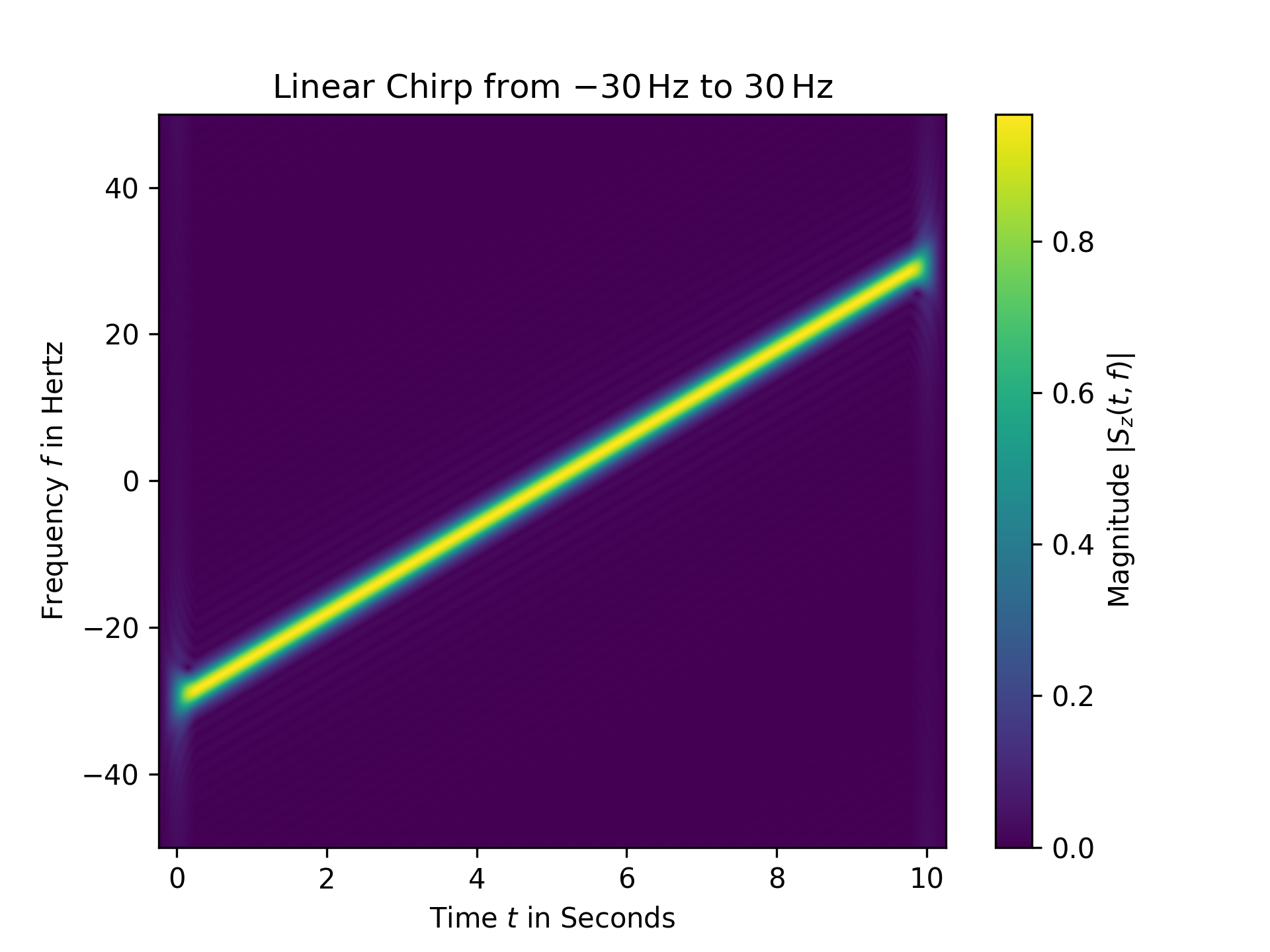
Finally, the short-time Fourier transform of a complex-valued linear chirp ranging from -30 Hz to 30 Hz is depicted:

z_lin = chirp(t, f0=-30, f1=30, t1=N*T, method="linear", complex=True)
SFT.fft_mode = 'centered'  # needed to work with complex signals
aSz = abs(SFT.stft(z_lin))
fg2, ax2 = plt.subplots()

✓

ax2.set_title(r"Linear Chirp from $-30\,$Hz to $30\,$Hz")
ax2.set(xlabel="Time $t$ in Seconds", ylabel="Frequency $f$ in Hertz")

✗

im2 = ax2.imshow(aSz, origin='lower', aspect='auto',
                 extent=SFT.extent(N), cmap='viridis')

✓

fg2.colorbar(im2, label='Magnitude $|S_z(t,f)|$')

✗

plt.show()

✓

Note that using negative frequencies makes only sense with complex-valued signals. Furthermore, the magnitude of the complex exponential function is one whereas the magnitude of the real-valued cosine function is only 1/2.

Aliases

scipy.signal.chirp