bundles / scipy 1.17.1 / scipy / signal / _waveforms / sweep_poly
function
scipy.signal._waveforms:sweep_poly
source: /scipy/signal/_waveforms.py :473
Signature
def sweep_poly ( t , poly , phi = 0 ) Summary
Frequency-swept cosine generator, with a time-dependent frequency.
Extended Summary
This function generates a sinusoidal function whose instantaneous frequency varies with time. The frequency at time t is given by the polynomial poly.
Parameters
t: ndarrayTimes at which to evaluate the waveform.
poly: 1-D array_like or instance of numpy.poly1dThe desired frequency expressed as a polynomial. If
polyis a list or ndarray of length n, then the elements ofpolyare the coefficients of the polynomial, and the instantaneous frequency isf(t) = poly[0]*t**(n-1) + poly[1]*t**(n-2) + ... + poly[n-1]If
polyis an instance of numpy.poly1d, then the instantaneous frequency isf(t) = poly(t)phi: float, optionalPhase offset, in degrees, Default: 0.
Returns
sweep_poly: ndarrayA numpy array containing the signal evaluated at
twith the requested time-varying frequency. More precisely, the function returnscos(phase + (pi/180)*phi), wherephaseis the integral (from 0 to t) of2 * pi * f(t);f(t)is defined above.
Notes
If poly is a list or ndarray of length n, then the elements of poly are the coefficients of the polynomial, and the instantaneous frequency is:
f(t) = poly[0]*t**(n-1) + poly[1]*t**(n-2) + ... + poly[n-1]
If poly is an instance of numpy.poly1d, then the instantaneous frequency is:
f(t) = poly(t)
Finally, the output s is:
cos(phase + (pi/180)*phi)
where phase is the integral from 0 to t of 2 * pi * f(t), f(t) as defined above.
Array API Standard Support
sweep_poly has experimental support for Python Array API Standard compatible backends in addition to NumPy. Please consider testing these features by setting an environment variable SCIPY_ARRAY_API=1 and providing CuPy, PyTorch, JAX, or Dask arrays as array arguments. The following combinations of backend and device (or other capability) are supported.
====================  ====================  ====================
Library               CPU                   GPU
====================  ====================  ====================
NumPy                 ✅                     n/a
CuPy                  n/a                   ⛔
PyTorch               ⛔                     ⛔
JAX                   ⛔                     ⛔
Dask                  ⛔                     n/a
====================  ====================  ====================
See
dev-arrayapifor more information.
Examples
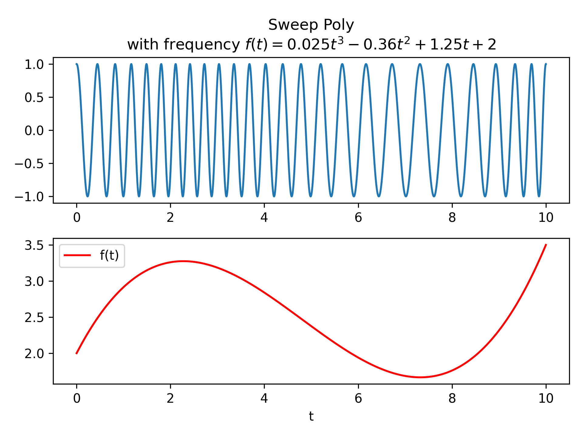
Compute the waveform with instantaneous frequency:: f(t) = 0.025*t**3 - 0.36*t**2 + 1.25*t + 2 over the interval 0 <= t <= 10.import numpy as np from scipy.signal import sweep_poly p = np.poly1d([0.025, -0.36, 1.25, 2.0]) t = np.linspace(0, 10, 5001) w = sweep_poly(t, p)✓
import matplotlib.pyplot as plt
✓plt.subplot(2, 1, 1) plt.plot(t, w) plt.title("Sweep Poly\nwith frequency " + "$f(t) = 0.025t^3 - 0.36t^2 + 1.25t + 2$") plt.subplot(2, 1, 2) plt.plot(t, p(t), 'r', label='f(t)') plt.legend() plt.xlabel('t')✗
plt.tight_layout()
plt.show()
✓
See also
Aliases
-
scipy.signal.sweep_poly