`scipy.stats._continuous_distns:kstwo_gen`

source: /scipy/stats/_continuous_distns.py :197

Signature

   class     kstwo_gen (    momtype    =  1   ,    a    =  None   ,    b    =  None   ,    xtol    =  1e-14   ,    badvalue    =  None   ,    name    =  None   ,    longname    =  None   ,    shapes    =  None   ,    seed    =  None     )

Members

Summary

Kolmogorov-Smirnov two-sided test statistic distribution.

Extended Summary

This is the distribution of the two-sided Kolmogorov-Smirnov (KS) statistic $D_{n}$ for a finite sample size n >= 1 (the shape parameter).

%(before_notes)s

Notes

$D_{n}$ is given by

D_{n} = sup_{x} ∣ F_{n} (x) - F (x) ∣

where $F$ is a (continuous) CDF and $F_{n}$ is an empirical CDF. kstwo describes the distribution under the null hypothesis of the KS test that the empirical CDF corresponds to $n$ i.i.d. random variates with CDF $F$ .

%(after_notes)s

Examples

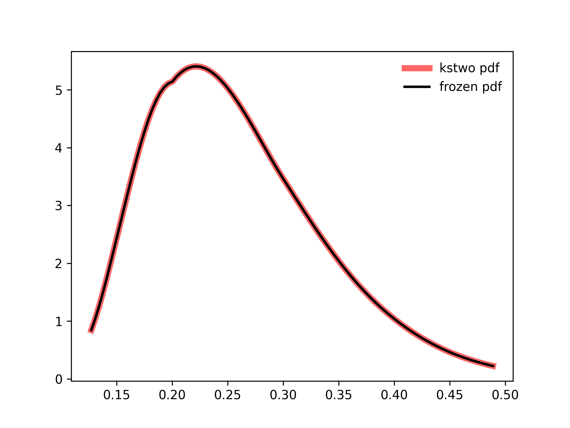
import numpy as np
from scipy.stats import kstwo
import matplotlib.pyplot as plt
fig, ax = plt.subplots(1, 1)

✓

Display the probability density function (``pdf``):

n = 10
x = np.linspace(kstwo.ppf(0.01, n),
                kstwo.ppf(0.99, n), 100)

✓

ax.plot(x, kstwo.pdf(x, n),
        'r-', lw=5, alpha=0.6, label='kstwo pdf')

✗

Alternatively, the distribution object can be called (as a function) to fix the shape, location and scale parameters. This returns a "frozen" RV object holding the given parameters fixed. Freeze the distribution and display the frozen ``pdf``:

rv = kstwo(n)

✓

ax.plot(x, rv.pdf(x), 'k-', lw=2, label='frozen pdf')
ax.legend(loc='best', frameon=False)

✗

plt.show()

✓

Check accuracy of ``cdf`` and ``ppf``:

vals = kstwo.ppf([0.001, 0.5, 0.999], n)
np.allclose([0.001, 0.5, 0.999], kstwo.cdf(vals, n))

✓

Aliases

scipy.stats._continuous_distns.kstwo_gen