bundles / scipy 1.17.1 / scipy / stats / _continuous_distns / levy_l_gen
class
scipy.stats._continuous_distns:levy_l_gen
Signature
class levy_l_gen ( momtype = 1 , a = None , b = None , xtol = 1e-14 , badvalue = None , name = None , longname = None , shapes = None , seed = None ) Members
Summary
A left-skewed Levy continuous random variable.
Extended Summary
%(before_notes)s
Notes
The probability density function for levy_l is:
for .
This is the same as the Levy-stable distribution with and .
%(after_notes)s
Examples
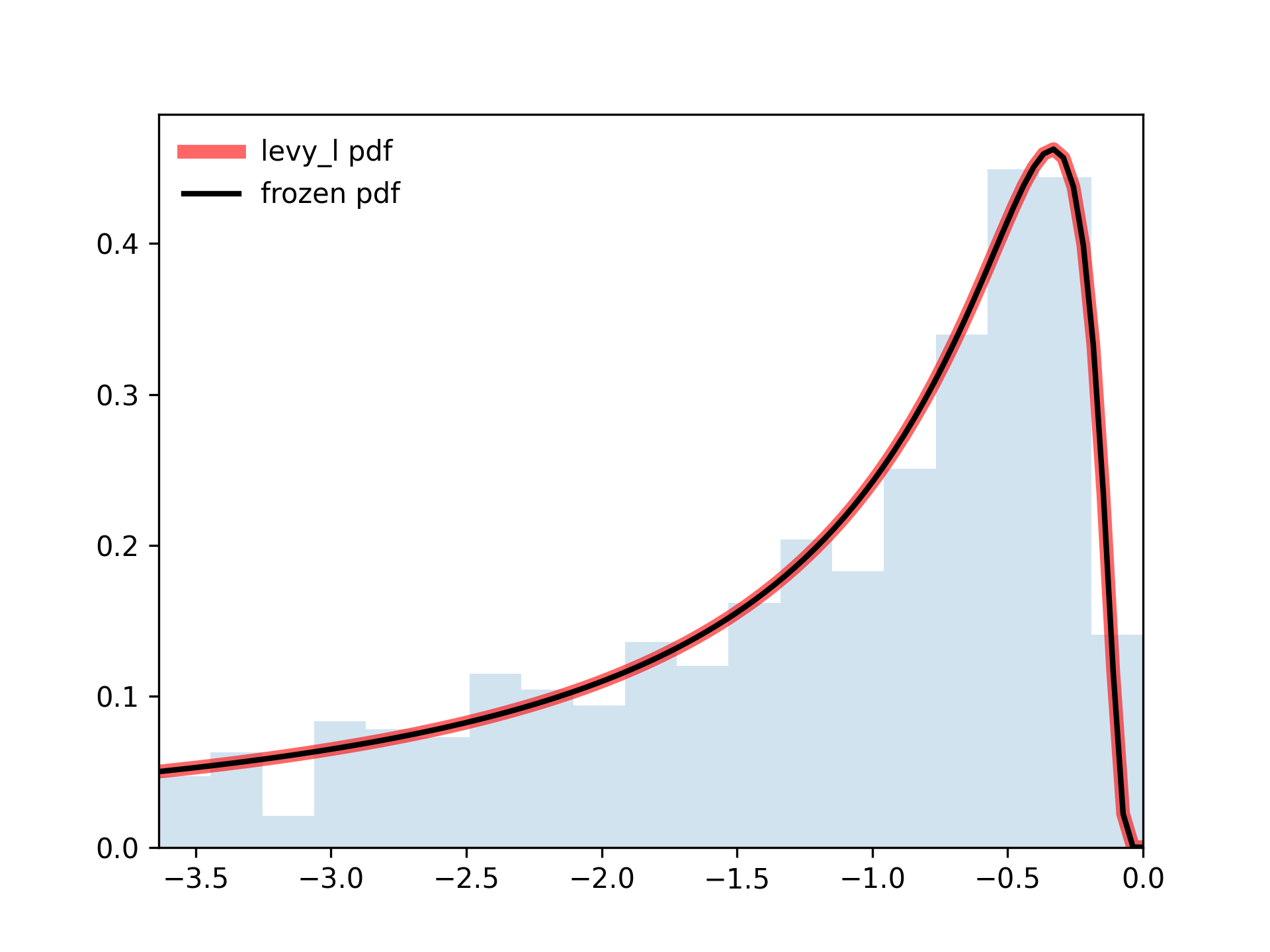
import numpy as np
from scipy.stats import levy_l
import matplotlib.pyplot as plt
fig, ax = plt.subplots(1, 1)
✓
mean, var, skew, kurt = levy_l.stats(moments='mvsk')
✓a, b = levy_l.ppf(0.4), levy_l.ppf(1) x = np.linspace(a, b, 100)✓
ax.plot(x, levy_l.pdf(x),
       'r-', lw=5, alpha=0.6, label='levy_l pdf')
✗
rv = levy_l()
✓ax.plot(x, rv.pdf(x), 'k-', lw=2, label='frozen pdf')
✗vals = levy_l.ppf([0.001, 0.5, 0.999]) np.allclose([0.001, 0.5, 0.999], levy_l.cdf(vals))✓
r = levy_l.rvs(size=1000)
✓bins = np.concatenate(([np.min(r)], np.linspace(a, b, 20)))
✓ax.hist(r, bins=bins, density=True, histtype='stepfilled', alpha=0.2) ax.set_xlim([x[0], x[-1]]) ax.legend(loc='best', frameon=False)✗
plt.show()
✓
See also
- levy
- levy_stable
Aliases
-
scipy.stats._continuous_distns.levy_l_gen