bundles / scipy latest / scipy / optimize / _lsq / least_squares / least_squares

function

`scipy.optimize._lsq.least_squares:least_squares`

source: /scipy/optimize/_lsq/least_squares.py :266

Signature

   def     least_squares (    fun    ,    x0    ,    jac    =  2-point   ,    bounds    =  (-inf, inf)   ,    method    =  trf   ,    ftol    =  1e-08   ,    xtol    =  1e-08   ,    gtol    =  1e-08   ,    x_scale    =  None   ,    loss    =  linear   ,    f_scale    =  1.0   ,    diff_step    =  None   ,    tr_solver    =  None   ,    tr_options    =  None   ,    jac_sparsity    =  None   ,    max_nfev    =  None   ,    verbose    =  0   ,    args    =  ()   ,    kwargs    =  None   ,    callback    =  None   ,    workers    =  None     )

Summary

Solve a nonlinear least-squares problem with bounds on the variables.

Extended Summary

Given the residuals f(x) (an m-D real function of n real variables) and the loss function rho(s) (a scalar function), least_squares finds a local minimum of the cost function F(x)

minimize F(x) = 0.5 * sum(rho(f_i(x)**2), i = 0, ..., m - 1)
subject to lb <= x <= ub

The purpose of the loss function rho(s) is to reduce the influence of outliers on the solution.

Parameters

fun : callable

Function which computes the vector of residuals, with the signature fun(x, *args, **kwargs), i.e., the minimization proceeds with respect to its first argument. The argument x passed to this function is an ndarray of shape (n,) (never a scalar, even for n=1). It must allocate and return a 1-D array_like of shape (m,) or a scalar. If the argument x is complex or the function fun returns complex residuals, it must be wrapped in a real function of real arguments, as shown at the end of the Examples section.

x0 : array_like with shape (n,) or float

Initial guess on independent variables. If float, it will be treated as a 1-D array with one element. When method is 'trf', the initial guess might be slightly adjusted to lie sufficiently within the given bounds.

jac : {'2-point', '3-point', 'cs', callable}, optional

Method of computing the Jacobian matrix (an m-by-n matrix, where element (i, j) is the partial derivative of f[i] with respect to x[j]). The keywords select a finite difference scheme for numerical estimation. The scheme '3-point' is more accurate, but requires twice as many operations as '2-point' (default). The scheme 'cs' uses complex steps, and while potentially the most accurate, it is applicable only when fun correctly handles complex inputs and can be analytically continued to the complex plane. If callable, it is used as jac(x, *args, **kwargs) and should return a good approximation (or the exact value) for the Jacobian as an array_like (np.atleast_2d is applied), a sparse array (csr_array preferred for performance) or a scipy.sparse.linalg.LinearOperator.

bounds : 2-tuple of array_like or `Bounds`, optional

There are two ways to specify bounds:

Instance of Bounds class
Lower and upper bounds on independent variables. Defaults to no bounds. Each array must match the size of x0 or be a scalar, in the latter case a bound will be the same for all variables. Use np.inf with an appropriate sign to disable bounds on all or some variables.

method : {'trf', 'dogbox', 'lm'}, optional

Algorithm to perform minimization.

'trf'Trust Region Reflective algorithm, particularly suitable for large sparse problems with bounds. Generally robust method.
'dogbox'dogleg algorithm with rectangular trust regions, typical use case is small problems with bounds. Not recommended for problems with rank-deficient Jacobian.
'lm'Levenberg-Marquardt algorithm as implemented in MINPACK. Doesn't handle bounds and sparse Jacobians. Usually the most efficient method for small unconstrained problems.

Default is 'trf'. See Notes for more information.

ftol : float or None, optional

Tolerance for termination by the change of the cost function. Default is 1e-8. The optimization process is stopped when dF < ftol * F, and there was an adequate agreement between a local quadratic model and the true model in the last step.

If None and 'method' is not 'lm', the termination by this condition is disabled. If 'method' is 'lm', this tolerance must be higher than machine epsilon.

xtol : float or None, optional

Tolerance for termination by the change of the independent variables. Default is 1e-8. The exact condition depends on the method used:

For 'trf' and 'dogbox'norm(dx) < xtol * (xtol + norm(x)).
For 'lm'Delta < xtol * norm(xs), where Delta is a trust-region radius and xs is the value of x scaled according to x_scale parameter (see below).

If None and 'method' is not 'lm', the termination by this condition is disabled. If 'method' is 'lm', this tolerance must be higher than machine epsilon.

gtol : float or None, optional

Tolerance for termination by the norm of the gradient. Default is 1e-8. The exact condition depends on a method used:

For 'trf'norm(g_scaled, ord=np.inf) < gtol, where g_scaled is the value of the gradient scaled to account for the presence of the bounds [STIR].
For 'dogbox'norm(g_free, ord=np.inf) < gtol, where g_free is the gradient with respect to the variables which are not in the optimal state on the boundary.
For 'lm'the maximum absolute value of the cosine of angles between columns of the Jacobian and the residual vector is less than gtol, or the residual vector is zero.

If None and 'method' is not 'lm', the termination by this condition is disabled. If 'method' is 'lm', this tolerance must be higher than machine epsilon.

x_scale : {None, array_like, 'jac'}, optional

Characteristic scale of each variable. Setting x_scale is equivalent to reformulating the problem in scaled variables xs = x / x_scale. An alternative view is that the size of a trust region along jth dimension is proportional to x_scale[j]. Improved convergence may be achieved by setting x_scale such that a step of a given size along any of the scaled variables has a similar effect on the cost function. If set to 'jac', the scale is iteratively updated using the inverse norms of the columns of the Jacobian matrix (as described in [JJMore]). The default scaling for each method (i.e. if x_scale is None) is as follows:

For 'trf'x_scale == 1
For 'dogbox'x_scale == 1
For 'lm'x_scale == 'jac'

loss : str or callable, optional

Determines the loss function. The following keyword values are allowed:

'linear' (default)rho(z) = z. Gives a standard least-squares problem.
'soft_l1'rho(z) = 2 * ((1 + z)**0.5 - 1). The smooth approximation of l1 (absolute value) loss. Usually a good choice for robust least squares.
'huber'rho(z) = z if z <= 1 else 2*z**0.5 - 1. Works similarly to 'soft_l1'.
'cauchy'rho(z) = ln(1 + z). Severely weakens outliers influence, but may cause difficulties in optimization process.
'arctan'rho(z) = arctan(z). Limits a maximum loss on a single residual, has properties similar to 'cauchy'.

If callable, it must take a 1-D ndarray z=f**2 and return an array_like with shape (3, m) where row 0 contains function values, row 1 contains first derivatives and row 2 contains second derivatives. Method 'lm' supports only 'linear' loss.

f_scale : float, optional

Value of soft margin between inlier and outlier residuals, default is 1.0. The loss function is evaluated as follows rho_(f**2) = C**2 * rho(f**2 / C**2), where C is f_scale, and rho is determined by loss parameter. This parameter has no effect with loss='linear', but for other loss values it is of crucial importance.

max_nfev : None or int, optional

For all methods this parameter controls the maximum number of function evaluations used by each method, separate to those used in numerical approximation of the jacobian. If None (default), the value is chosen automatically as 100 * n.

diff_step : None or array_like, optional

Determines the relative step size for the finite difference approximation of the Jacobian. The actual step is computed as x * diff_step. If None (default), then diff_step is taken to be a conventional "optimal" power of machine epsilon for the finite difference scheme used [NR].

tr_solver : {None, 'exact', 'lsmr'}, optional

Method for solving trust-region subproblems, relevant only for 'trf' and 'dogbox' methods.

'exact' is suitable for not very large problems with dense Jacobian matrices. The computational complexity per iteration is comparable to a singular value decomposition of the Jacobian matrix.
'lsmr' is suitable for problems with sparse and large Jacobian matrices. It uses the iterative procedure scipy.sparse.linalg.lsmr for finding a solution of a linear least-squares problem and only requires matrix-vector product evaluations.

If None (default), the solver is chosen based on the type of Jacobian returned on the first iteration.

tr_options : dict, optional

Keyword options passed to trust-region solver.

tr_solver='exact': tr_options are ignored.
tr_solver='lsmr': options for scipy.sparse.linalg.lsmr. Additionally, method='trf' supports 'regularize' option (bool, default is True), which adds a regularization term to the normal equation, which improves convergence if the Jacobian is rank-deficient [Byrd] (eq. 3.4).

jac_sparsity : {None, array_like, sparse array}, optional

Defines the sparsity structure of the Jacobian matrix for finite difference estimation, its shape must be (m, n). If the Jacobian has only few non-zero elements in each row, providing the sparsity structure will greatly speed up the computations [Curtis]. A zero entry means that a corresponding element in the Jacobian is identically zero. If provided, forces the use of 'lsmr' trust-region solver. If None (default), then dense differencing will be used. Has no effect for 'lm' method.

verbose : {0, 1, 2}, optional

Level of algorithm's verbosity:

0 (default)work silently.
1display a termination report.
2display progress during iterations (not supported by 'lm' method).

args, kwargs : tuple and dict, optional

Additional arguments passed to fun and jac. Both empty by default. The calling signature is fun(x, *args, **kwargs) and the same for jac.

callback : None or callable, optional

Callback function that is called by the algorithm on each iteration. This can be used to print or plot the optimization results at each step, and to stop the optimization algorithm based on some user-defined condition. Only implemented for the trf and dogbox methods.

The signature is callback(intermediate_result: OptimizeResult)

intermediate_result is a 'scipy.optimize.OptimizeResult which contains the intermediate results of the optimization at the current iteration.

The callback also supports a signature like: callback(x)

Introspection is used to determine which of the signatures is invoked.

If the callback function raises StopIteration the optimization algorithm will stop and return with status code -2.

workers : map-like callable, optional

A map-like callable, such as multiprocessing.Pool.map for evaluating any numerical differentiation in parallel. This evaluation is carried out as workers(fun, iterable).

Returns

result : OptimizeResult

OptimizeResult with the following fields defined:

x: x
cost: cost
fun: fun
jac: jac
grad: grad
optimality: optimality
active_mask: active_mask
nfev: nfev
njev: njev
status: status
message: message
success: success

Notes

Method 'lm' (Levenberg-Marquardt) calls a wrapper over a least-squares algorithm implemented in MINPACK (lmder). It runs the Levenberg-Marquardt algorithm formulated as a trust-region type algorithm. The implementation is based on paper [JJMore], it is very robust and efficient with a lot of smart tricks. It should be your first choice for unconstrained problems. Note that it doesn't support bounds. Also, it doesn't work when m < n.

Method 'trf' (Trust Region Reflective) is motivated by the process of solving a system of equations, which constitute the first-order optimality condition for a bound-constrained minimization problem as formulated in [STIR]. The algorithm iteratively solves trust-region subproblems augmented by a special diagonal quadratic term and with trust-region shape determined by the distance from the bounds and the direction of the gradient. This enhancements help to avoid making steps directly into bounds and efficiently explore the whole space of variables. To further improve convergence, the algorithm considers search directions reflected from the bounds. To obey theoretical requirements, the algorithm keeps iterates strictly feasible. With dense Jacobians trust-region subproblems are solved by an exact method very similar to the one described in [JJMore] (and implemented in MINPACK). The difference from the MINPACK implementation is that a singular value decomposition of a Jacobian matrix is done once per iteration, instead of a QR decomposition and series of Givens rotation eliminations. For large sparse Jacobians a 2-D subspace approach of solving trust-region subproblems is used [STIR], [Byrd]. The subspace is spanned by a scaled gradient and an approximate Gauss-Newton solution delivered by scipy.sparse.linalg.lsmr. When no constraints are imposed the algorithm is very similar to MINPACK and has generally comparable performance. The algorithm works quite robust in unbounded and bounded problems, thus it is chosen as a default algorithm.

Method 'dogbox' operates in a trust-region framework, but considers rectangular trust regions as opposed to conventional ellipsoids [Voglis]. The intersection of a current trust region and initial bounds is again rectangular, so on each iteration a quadratic minimization problem subject to bound constraints is solved approximately by Powell's dogleg method [NumOpt]. The required Gauss-Newton step can be computed exactly for dense Jacobians or approximately by scipy.sparse.linalg.lsmr for large sparse Jacobians. The algorithm is likely to exhibit slow convergence when the rank of Jacobian is less than the number of variables. The algorithm often outperforms 'trf' in bounded problems with a small number of variables.

Robust loss functions are implemented as described in [BA]. The idea is to modify a residual vector and a Jacobian matrix on each iteration such that computed gradient and Gauss-Newton Hessian approximation match the true gradient and Hessian approximation of the cost function. Then the algorithm proceeds in a normal way, i.e., robust loss functions are implemented as a simple wrapper over standard least-squares algorithms.

Examples

In this example we find a minimum of the Rosenbrock function without bounds on independent variables.

import numpy as np
def fun_rosenbrock(x):
    return np.array([10 * (x[1] - x[0]**2), (1 - x[0])])

✓

Notice that we only provide the vector of the residuals. The algorithm constructs the cost function as a sum of squares of the residuals, which gives the Rosenbrock function. The exact minimum is at ``x = [1.0, 1.0]``.

from scipy.optimize import least_squares
x0_rosenbrock = np.array([2, 2])
res_1 = least_squares(fun_rosenbrock, x0_rosenbrock)

✓

res_1.x
res_1.cost
res_1.optimality

✗

We now constrain the variables, in such a way that the previous solution becomes infeasible. Specifically, we require that ``x[1] >= 1.5``, and ``x[0]`` left unconstrained. To this end, we specify the `bounds` parameter to `least_squares` in the form ``bounds=([-np.inf, 1.5], np.inf)``. We also provide the analytic Jacobian:

def jac_rosenbrock(x):
    return np.array([
        [-20 * x[0], 10],
        [-1, 0]])

✓

Putting this all together, we see that the new solution lies on the bound:

res_2 = least_squares(fun_rosenbrock, x0_rosenbrock, jac_rosenbrock,
                      bounds=([-np.inf, 1.5], np.inf))

✓

res_2.x
res_2.cost
res_2.optimality

✗

Now we solve a system of equations (i.e., the cost function should be zero at a minimum) for a Broyden tridiagonal vector-valued function of 100000 variables:

def fun_broyden(x):
    f = (3 - x) * x + 1
    f[1:] -= x[:-1]
    f[:-1] -= 2 * x[1:]
    return f

✓

The corresponding Jacobian matrix is sparse. We tell the algorithm to estimate it by finite differences and provide the sparsity structure of Jacobian to significantly speed up this process.

from scipy.sparse import lil_array
def sparsity_broyden(n):
    sparsity = lil_array((n, n), dtype=int)
    i = np.arange(n)
    sparsity[i, i] = 1
    i = np.arange(1, n)
    sparsity[i, i - 1] = 1
    i = np.arange(n - 1)
    sparsity[i, i + 1] = 1
    return sparsity
n = 100000
x0_broyden = -np.ones(n)
res_3 = least_squares(fun_broyden, x0_broyden,
                      jac_sparsity=sparsity_broyden(n))

✓

res_3.cost
res_3.optimality

✗

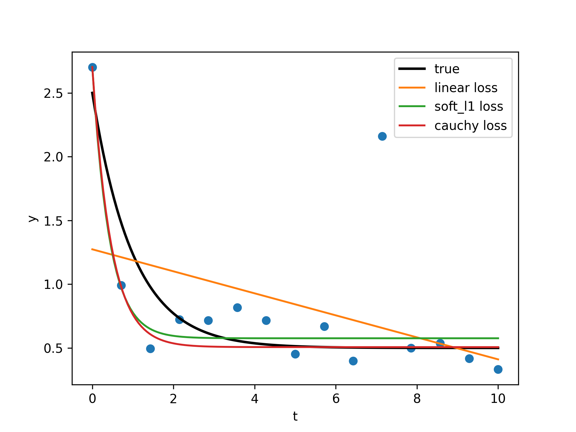
Let's also solve a curve fitting problem using robust loss function to take care of outliers in the data. Define the model function as ``y = a + b * exp(c * t)``, where t is a predictor variable, y is an observation and a, b, c are parameters to estimate. First, define the function which generates the data with noise and outliers, define the model parameters, and generate data:

from numpy.random import default_rng
rng = default_rng()
def gen_data(t, a, b, c, noise=0., n_outliers=0, seed=None):
    rng = default_rng(seed)

    y = a + b * np.exp(t * c)

    error = noise * rng.standard_normal(t.size)
    outliers = rng.integers(0, t.size, n_outliers)
    error[outliers] *= 10

    return y + error
a = 0.5
b = 2.0
c = -1
t_min = 0
t_max = 10
n_points = 15
t_train = np.linspace(t_min, t_max, n_points)
y_train = gen_data(t_train, a, b, c, noise=0.1, n_outliers=3)

✓

Define function for computing residuals and initial estimate of parameters.

def fun(x, t, y):
    return x[0] + x[1] * np.exp(x[2] * t) - y
x0 = np.array([1.0, 1.0, 0.0])

✓

Compute a standard least-squares solution:

res_lsq = least_squares(fun, x0, args=(t_train, y_train))

✓

Now compute two solutions with two different robust loss functions. The parameter `f_scale` is set to 0.1, meaning that inlier residuals should not significantly exceed 0.1 (the noise level used).

res_soft_l1 = least_squares(fun, x0, loss='soft_l1', f_scale=0.1,
                            args=(t_train, y_train))
res_log = least_squares(fun, x0, loss='cauchy', f_scale=0.1,
                        args=(t_train, y_train))

✓

And, finally, plot all the curves. We see that by selecting an appropriate `loss` we can get estimates close to optimal even in the presence of strong outliers. But keep in mind that generally it is recommended to try 'soft_l1' or 'huber' losses first (if at all necessary) as the other two options may cause difficulties in optimization process.

t_test = np.linspace(t_min, t_max, n_points * 10)
y_true = gen_data(t_test, a, b, c)
y_lsq = gen_data(t_test, *res_lsq.x)
y_soft_l1 = gen_data(t_test, *res_soft_l1.x)
y_log = gen_data(t_test, *res_log.x)
import matplotlib.pyplot as plt

✓

plt.plot(t_train, y_train, 'o')
plt.plot(t_test, y_true, 'k', linewidth=2, label='true')
plt.plot(t_test, y_lsq, label='linear loss')
plt.plot(t_test, y_soft_l1, label='soft_l1 loss')
plt.plot(t_test, y_log, label='cauchy loss')
plt.xlabel("t")
plt.ylabel("y")
plt.legend()

✗

plt.show()

✓

In the next example, we show how complex-valued residual functions of complex variables can be optimized with ``least_squares()``. Consider the following function:

def f(z):
    return z - (0.5 + 0.5j)

✓

We wrap it into a function of real variables that returns real residuals by simply handling the real and imaginary parts as independent variables:

def f_wrap(x):
    fx = f(x[0] + 1j*x[1])
    return np.array([fx.real, fx.imag])

✓

Thus, instead of the original m-D complex function of n complex variables we optimize a 2m-D real function of 2n real variables:

from scipy.optimize import least_squares
res_wrapped = least_squares(f_wrap, (0.1, 0.1), bounds=([0, 0], [1, 1]))
z = res_wrapped.x[0] + res_wrapped.x[1]*1j

✓

✗

Aliases

scipy.optimize.least_squares

`scipy.optimize._lsq.least_squares:least_squares`

Signature

Summary

Extended Summary

Parameters

Returns

Notes

Examples

See also

Aliases

Referenced by

This package