bundles / scipy latest / scipy / stats / _fit / fit

function

`scipy.stats._fit:fit`

source: /scipy/stats/_fit.py :317

Signature

   def     fit (    dist    ,    data    ,    bounds    =  None   ,  * ,     guess    =  None   ,    method    =  mle   ,    optimizer    =  <function differential_evolution at 0x0000>     )

Summary

Fit a discrete or continuous distribution to data

Extended Summary

Given a distribution, data, and bounds on the parameters of the distribution, return maximum likelihood estimates of the parameters.

Parameters

dist : `scipy.stats.rv_continuous` or `scipy.stats.rv_discrete`

The object representing the distribution to be fit to the data.

data : 1D array_like

The data to which the distribution is to be fit. If the data contain any of np.nan, np.inf, or -np.inf, the fit method will raise a ValueError.

bounds : dict or sequence of tuples, optional

If a dictionary, each key is the name of a parameter of the distribution, and the corresponding value is a tuple containing the lower and upper bound on that parameter. If the distribution is defined only for a finite range of values of that parameter, no entry for that parameter is required; e.g., some distributions have parameters which must be on the interval [0, 1]. Bounds for parameters location (loc) and scale (scale) are optional; by default, they are fixed to 0 and 1, respectively.

If a sequence, element i is a tuple containing the lower and upper bound on the ith parameter of the distribution. In this case, bounds for all distribution shape parameters must be provided. Optionally, bounds for location and scale may follow the distribution shape parameters.

If a shape is to be held fixed (e.g. if it is known), the lower and upper bounds may be equal. If a user-provided lower or upper bound is beyond a bound of the domain for which the distribution is defined, the bound of the distribution's domain will replace the user-provided value. Similarly, parameters which must be integral will be constrained to integral values within the user-provided bounds.

guess : dict or array_like, optional

If a dictionary, each key is the name of a parameter of the distribution, and the corresponding value is a guess for the value of the parameter.

If a sequence, element i is a guess for the ith parameter of the distribution. In this case, guesses for all distribution shape parameters must be provided.

If guess is not provided, guesses for the decision variables will not be passed to the optimizer. If guess is provided, guesses for any missing parameters will be set at the mean of the lower and upper bounds. Guesses for parameters which must be integral will be rounded to integral values, and guesses that lie outside the intersection of the user-provided bounds and the domain of the distribution will be clipped.

method : {'mle', 'mse'}

With method="mle" (default), the fit is computed by minimizing the negative log-likelihood function. A large, finite penalty (rather than infinite negative log-likelihood) is applied for observations beyond the support of the distribution. With method="mse", the fit is computed by minimizing the negative log-product spacing function. The same penalty is applied for observations beyond the support. We follow the approach of ^[1], which is generalized for samples with repeated observations.

optimizer : callable, optional

optimizer is a callable that accepts the following positional argument.

fun: fun

optimizer must also accept the following keyword argument.

bounds: bounds

If guess is provided, optimizer must also accept the following keyword argument.

x0: x0

If the distribution has any shape parameters that must be integral or if the distribution is discrete and the location parameter is not fixed, optimizer must also accept the following keyword argument.

integrality: integrality

optimizer must return an object, such as an instance of scipy.optimize.OptimizeResult, which holds the optimal values of the decision variables in an attribute x. If attributes fun, status, or message are provided, they will be included in the result object returned by fit.

Returns

result : `~scipy.stats._result_classes.FitResult`

An object with the following fields.

params: params
success: success
message: message

The object has the following method:

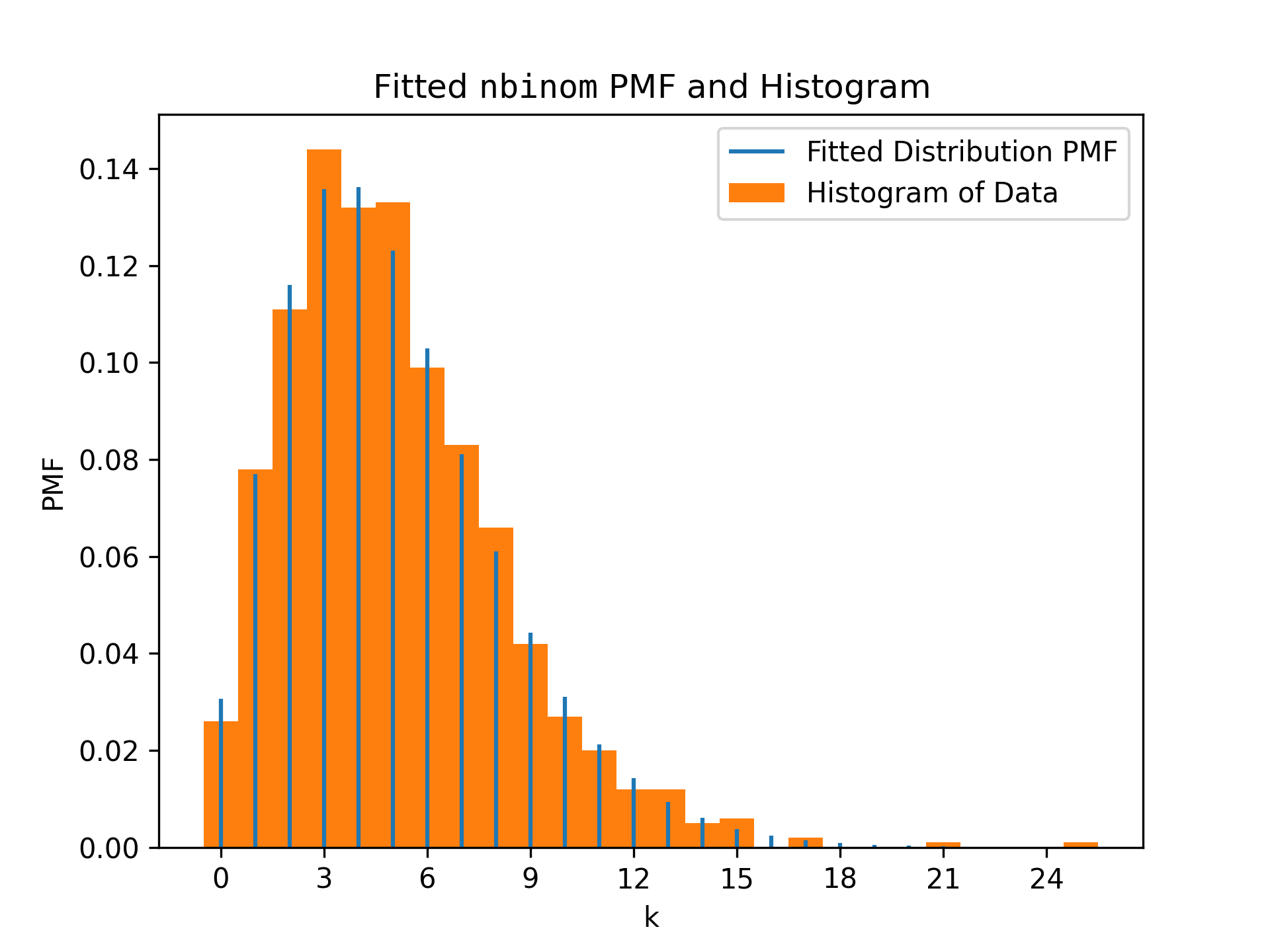
nllf(params=None, data=None): By default, the negative log-likelihood function at the fitted params for the given data. Accepts a tuple containing alternative shapes, location, and scale of the distribution and an array of alternative data.
plot(ax=None): Superposes the PDF/PMF of the fitted distribution over a normalized histogram of the data.

Notes

Optimization is more likely to converge to the maximum likelihood estimate when the user provides tight bounds containing the maximum likelihood estimate. For example, when fitting a binomial distribution to data, the number of experiments underlying each sample may be known, in which case the corresponding shape parameter n can be fixed.

Array API Standard Support

fit is not in-scope for support of Python Array API Standard compatible backends other than NumPy.

See dev-arrayapi for more information.

Examples

Suppose we wish to fit a distribution to the following data.

import numpy as np
from scipy import stats
rng = np.random.default_rng()
dist = stats.nbinom
shapes = (5, 0.5)
data = dist.rvs(*shapes, size=1000, random_state=rng)

✓

Suppose we do not know how the data were generated, but we suspect that it follows a negative binomial distribution with parameters *n* and *p*\. (See `scipy.stats.nbinom`.) We believe that the parameter *n* was fewer than 30, and we know that the parameter *p* must lie on the interval [0, 1]. We record this information in a variable `bounds` and pass this information to `fit`.

bounds = [(0, 30), (0, 1)]
res = stats.fit(dist, data, bounds)

✓

`fit` searches within the user-specified `bounds` for the values that best match the data (in the sense of maximum likelihood estimation). In this case, it found shape values similar to those from which the data were actually generated.

res.params

✗

We can visualize the results by superposing the probability mass function of the distribution (with the shapes fit to the data) over a normalized histogram of the data.

import matplotlib.pyplot as plt  # matplotlib must be installed to plot

✓

res.plot()

✗

plt.show()

✓

Note that the estimate for *n* was exactly integral; this is because the domain of the `nbinom` PMF includes only integral *n*, and the `nbinom` object "knows" that. `nbinom` also knows that the shape *p* must be a value between 0 and 1. In such a case - when the domain of the distribution with respect to a parameter is finite - we are not required to specify bounds for the parameter.

bounds = {'n': (0, 30)}  # omit parameter p using a `dict`
res2 = stats.fit(dist, data, bounds)

✓

res2.params

✗

If we wish to force the distribution to be fit with *n* fixed at 6, we can set both the lower and upper bounds on *n* to 6. Note, however, that the value of the objective function being optimized is typically worse (higher) in this case.

bounds = {'n': (6, 6)}  # fix parameter `n`
res3 = stats.fit(dist, data, bounds)

✓

res3.params
res3.nllf() > res.nllf()

✗

Note that the numerical results of the previous examples are typical, but they may vary because the default optimizer used by `fit`, `scipy.optimize.differential_evolution`, is stochastic. However, we can customize the settings used by the optimizer to ensure reproducibility - or even use a different optimizer entirely - using the `optimizer` parameter.

from scipy.optimize import differential_evolution
rng = np.random.default_rng(767585560716548)
def optimizer(fun, bounds, *, integrality):
    return differential_evolution(fun, bounds, strategy='best2bin',
                                  rng=rng, integrality=integrality)
bounds = [(0, 30), (0, 1)]
res4 = stats.fit(dist, data, bounds, optimizer=optimizer)

✓

res4.params

`scipy.stats._fit:fit`

Signature

Summary

Extended Summary

Parameters

Returns

Notes

Examples

See also

Aliases

Referenced by

This package