bundles / scipy latest / scipy / stats / _fit / goodness_of_fit

function

`scipy.stats._fit:goodness_of_fit`

source: /scipy/stats/_fit.py :743

Signature

   def     goodness_of_fit (    dist    ,    data    ,  * ,     known_params    =  None   ,    fit_params    =  None   ,    guessed_params    =  None   ,    statistic    =  ad   ,    n_mc_samples    =  9999   ,    rng    =  None   ,    random_state    =  None     )

Summary

Perform a goodness of fit test comparing data to a distribution family.

Extended Summary

Given a distribution family and data, perform a test of the null hypothesis that the data were drawn from a distribution in that family. Any known parameters of the distribution may be specified. Remaining parameters of the distribution will be fit to the data, and the p-value of the test is computed accordingly. Several statistics for comparing the distribution to data are available.

Parameters

dist : `scipy.stats.rv_continuous`

The object representing the distribution family under the null hypothesis.

data : 1D array_like

Finite, uncensored data to be tested.

known_params : dict, optional

A dictionary containing name-value pairs of known distribution parameters. Monte Carlo samples are randomly drawn from the null-hypothesized distribution with these values of the parameters. Before the statistic is evaluated for the observed data and each Monte Carlo sample, only remaining unknown parameters of the null-hypothesized distribution family are fit to the samples; the known parameters are held fixed. If all parameters of the distribution family are known, then the step of fitting the distribution family to each sample is omitted.

fit_params : dict, optional

A dictionary containing name-value pairs of distribution parameters that have already been fit to the data, e.g. using scipy.stats.fit or the fit method of dist. Monte Carlo samples are drawn from the null-hypothesized distribution with these specified values of the parameter. However, these and all other unknown parameters of the null-hypothesized distribution family are always fit to the sample, whether that is the observed data or a Monte Carlo sample, before the statistic is evaluated.

guessed_params : dict, optional

A dictionary containing name-value pairs of distribution parameters which have been guessed. These parameters are always considered as free parameters and are fit both to the provided data as well as to the Monte Carlo samples drawn from the null-hypothesized distribution. The purpose of these guessed_params is to be used as initial values for the numerical fitting procedure.

statistic : {"ad", "ks", "cvm", "filliben"} or callable, optional

The statistic used to compare data to a distribution after fitting unknown parameters of the distribution family to the data. The Anderson-Darling ("ad") ^[1], Kolmogorov-Smirnov ("ks") ^[1], Cramer-von Mises ("cvm") ^[1], and Filliben ("filliben") ^[7] statistics are available. Alternatively, a callable with signature (dist, data, axis) may be supplied to compute the statistic. Here dist is a frozen distribution object (potentially with array parameters), data is an array of Monte Carlo samples (of compatible shape), and axis is the axis of data along which the statistic must be computed.

n_mc_samples : int, default: 9999

The number of Monte Carlo samples drawn from the null hypothesized distribution to form the null distribution of the statistic. The sample size of each is the same as the given data.

rng : {None, int, `numpy.random.Generator`}, optional

If rng is passed by keyword, types other than numpy.random.Generator are passed to numpy.random.default_rng to instantiate a Generator. If rng is already a Generator instance, then the provided instance is used. Specify rng for repeatable function behavior.

If this argument is passed by position or random_state is passed by keyword, legacy behavior for the argument random_state applies:

If random_state is None (or numpy.random), the numpy.random.RandomState singleton is used.
If random_state is an int, a new RandomState instance is used, seeded with random_state.
If random_state is already a Generator or RandomState instance then that instance is used.

Returns

res : GoodnessOfFitResult

An object with the following attributes.

fit_result: fit_result
statistic: statistic
pvalue: pvalue
null_distribution: null_distribution

Notes

This is a generalized Monte Carlo goodness-of-fit procedure, special cases of which correspond with various Anderson-Darling tests, Lilliefors' test, etc. The test is described in ^[2], ^[3], and ^[4] as a parametric bootstrap test. This is a Monte Carlo test in which parameters that specify the distribution from which samples are drawn have been estimated from the data. We describe the test using "Monte Carlo" rather than "parametric bootstrap" throughout to avoid confusion with the more familiar nonparametric bootstrap, and describe how the test is performed below.

Traditional goodness of fit tests

Traditionally, critical values corresponding with a fixed set of significance levels are pre-calculated using Monte Carlo methods. Users perform the test by calculating the value of the test statistic only for their observed data and comparing this value to tabulated critical values. This practice is not very flexible, as tables are not available for all distributions and combinations of known and unknown parameter values. Also, results can be inaccurate when critical values are interpolated from limited tabulated data to correspond with the user's sample size and fitted parameter values. To overcome these shortcomings, this function allows the user to perform the Monte Carlo trials adapted to their particular data.

Algorithmic overview

In brief, this routine executes the following steps:

Fit unknown parameters to the given data, thereby forming the "null-hypothesized" distribution, and compute the statistic of this pair of data and distribution.
Draw random samples from this null-hypothesized distribution.
Fit the unknown parameters to each random sample.
Calculate the statistic between each sample and the distribution that has been fit to the sample.
Compare the value of the statistic corresponding with data from (1) against the values of the statistic corresponding with the random samples from (4). The p-value is the proportion of samples with a statistic value greater than or equal to the statistic of the observed data.

In more detail, the steps are as follows.

First, any unknown parameters of the distribution family specified by dist are fit to the provided data using maximum likelihood estimation. (One exception is the normal distribution with unknown location and scale: we use the bias-corrected standard deviation np.std(data, ddof=1) for the scale as recommended in ^[1].) These values of the parameters specify a particular member of the distribution family referred to as the "null-hypothesized distribution", that is, the distribution from which the data were sampled under the null hypothesis. The statistic, which compares data to a distribution, is computed between data and the null-hypothesized distribution.

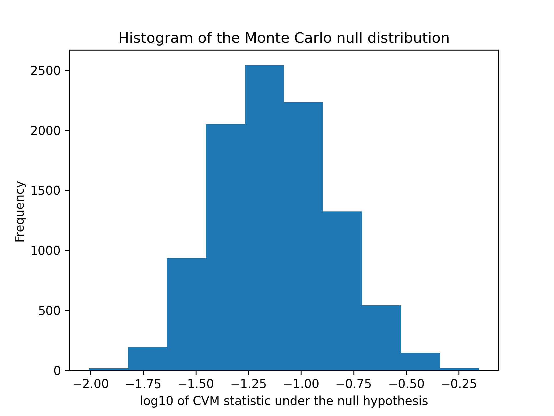
Next, many (specifically n_mc_samples) new samples, each containing the same number of observations as data, are drawn from the null-hypothesized distribution. All unknown parameters of the distribution family dist are fit to each resample, and the statistic is computed between each sample and its corresponding fitted distribution. These values of the statistic form the Monte Carlo null distribution (not to be confused with the "null-hypothesized distribution" above).

The p-value of the test is the proportion of statistic values in the Monte Carlo null distribution that are at least as extreme as the statistic value of the provided data. More precisely, the p-value is given by

p = \frac{b + 1}{m + 1}

where $b$ is the number of statistic values in the Monte Carlo null distribution that are greater than or equal to the statistic value calculated for data, and $m$ is the number of elements in the Monte Carlo null distribution (n_mc_samples). The addition of $1$ to the numerator and denominator can be thought of as including the value of the statistic corresponding with data in the null distribution, but a more formal explanation is given in ^[5].

Limitations

The test can be very slow for some distribution families because unknown parameters of the distribution family must be fit to each of the Monte Carlo samples, and for most distributions in SciPy, distribution fitting performed via numerical optimization.

Anti-Pattern

For this reason, it may be tempting to treat parameters of the distribution pre-fit to data (by the user) as though they were known_params, as specification of all parameters of the distribution precludes the need to fit the distribution to each Monte Carlo sample. (This is essentially how the original Kilmogorov-Smirnov test is performed.) Although such a test can provide evidence against the null hypothesis, the test is conservative in the sense that small p-values will tend to (greatly) overestimate the probability of making a type I error (that is, rejecting the null hypothesis although it is true), and the power of the test is low (that is, it is less likely to reject the null hypothesis even when the null hypothesis is false). This is because the Monte Carlo samples are less likely to agree with the null-hypothesized distribution as well as data. This tends to increase the values of the statistic recorded in the null distribution, so that a larger number of them exceed the value of statistic for data, thereby inflating the p-value.

Array API Standard Support

goodness_of_fit is not in-scope for support of Python Array API Standard compatible backends other than NumPy.

See dev-arrayapi for more information.

Examples

A well-known test of the null hypothesis that data were drawn from a given distribution is the Kolmogorov-Smirnov (KS) test, available in SciPy as `scipy.stats.ks_1samp`. Suppose we wish to test whether the following data:

import numpy as np
from scipy import stats
rng = np.random.default_rng(1638083107694713882823079058616272161)
x = stats.uniform.rvs(size=75, random_state=rng)

✓

were sampled from a normal distribution. To perform a KS test, the empirical distribution function of the observed data will be compared against the (theoretical) cumulative distribution function of a normal distribution. Of course, to do this, the normal distribution under the null hypothesis must be fully specified. This is commonly done by first fitting the ``loc`` and ``scale`` parameters of the distribution to the observed data, then performing the test.

loc, scale = np.mean(x), np.std(x, ddof=1)
cdf = stats.norm(loc, scale).cdf

✓

stats.ks_1samp(x, cdf)

✗

An advantage of the KS-test is that the p-value - the probability of obtaining a value of the test statistic under the null hypothesis as extreme as the value obtained from the observed data - can be calculated exactly and efficiently. `goodness_of_fit` can only approximate these results.

known_params = {'loc': loc, 'scale': scale}
res = stats.goodness_of_fit(stats.norm, x, known_params=known_params,
                            statistic='ks', rng=rng)

✓

res.statistic, res.pvalue

✗

The statistic matches exactly, but the p-value is estimated by forming a "Monte Carlo null distribution", that is, by explicitly drawing random samples from `scipy.stats.norm` with the provided parameters and calculating the stastic for each. The fraction of these statistic values at least as extreme as ``res.statistic`` approximates the exact p-value calculated by `scipy.stats.ks_1samp`. However, in many cases, we would prefer to test only that the data were sampled from one of *any* member of the normal distribution family, not specifically from the normal distribution with the location and scale fitted to the observed sample. In this case, Lilliefors [6]_ argued that the KS test is far too conservative (that is, the p-value overstates the actual probability of rejecting a true null hypothesis) and thus lacks power - the ability to reject the null hypothesis when the null hypothesis is actually false. Indeed, our p-value above is approximately 0.28, which is far too large to reject the null hypothesis at any common significance level. Consider why this might be. Note that in the KS test above, the statistic always compares data against the CDF of a normal distribution fitted to the *observed data*. This tends to reduce the value of the statistic for the observed data, but it is "unfair" when computing the statistic for other samples, such as those we randomly draw to form the Monte Carlo null distribution. It is easy to correct for this: whenever we compute the KS statistic of a sample, we use the CDF of a normal distribution fitted to *that sample*. The null distribution in this case has not been calculated exactly and is tyically approximated using Monte Carlo methods as described above. This is where `goodness_of_fit` excels.

res = stats.goodness_of_fit(stats.norm, x, statistic='ks', rng=rng)

✓

res.statistic, res.pvalue

✗

Indeed, this p-value is much smaller, and small enough to (correctly) reject the null hypothesis at common significance levels, including 5% and 2.5%. However, the KS statistic is not very sensitive to all deviations from normality. The original advantage of the KS statistic was the ability to compute the null distribution theoretically, but a more sensitive statistic - resulting in a higher test power - can be used now that we can approximate the null distribution computationally. The Anderson-Darling statistic [1]_ tends to be more sensitive, and critical values of this statistic have been tabulated for various significance levels and sample sizes using Monte Carlo methods.

res = stats.anderson(x, 'norm', method='interpolate')
print(res.statistic)
print(res.pvalue)

✓

Here, the observed value of the statistic exceeds the critical value corresponding with a 1% significance level. This tells us that the p-value of the observed data is 1% or less, but what is it? `goodness_of_fit` can estimate it directly.

res = stats.goodness_of_fit(stats.norm, x, statistic='ad', rng=rng)

✓

res.statistic, res.pvalue

✗

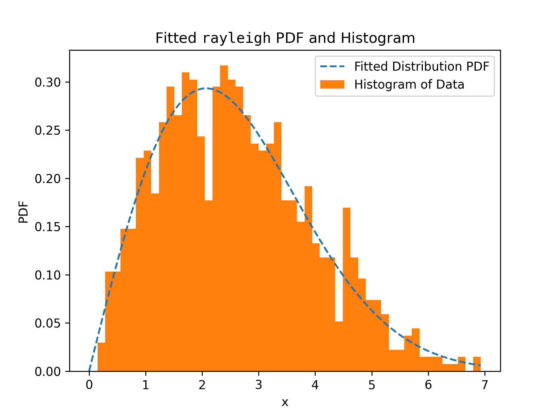
A further advantage is that use of `goodness_of_fit` is not limited to a particular set of distributions or conditions on which parameters are known versus which must be estimated from data. Instead, `goodness_of_fit` can estimate p-values relatively quickly for any distribution with a sufficiently fast and reliable ``fit`` method. For instance, here we perform a goodness of fit test using the Cramer-von Mises statistic against the Rayleigh distribution with known location and unknown scale.

rng = np.random.default_rng()
x = stats.chi(df=2.2, loc=0, scale=2).rvs(size=1000, random_state=rng)
res = stats.goodness_of_fit(stats.rayleigh, x, statistic='cvm',
                            known_params={'loc': 0}, rng=rng)

✓

This executes fairly quickly, but to check the reliability of the ``fit`` method, we should inspect the fit result.

res.fit_result  # location is as specified, and scale is reasonable

✗

import matplotlib.pyplot as plt  # matplotlib must be installed to plot

✓

res.fit_result.plot()

✗

plt.show()

✓

If the distribution is not fit to the observed data as well as possible, the test may not control the type I error rate, that is, the chance of rejecting the null hypothesis even when it is true. We should also look for extreme outliers in the null distribution that may be caused by unreliable fitting. These do not necessarily invalidate the result, but they tend to reduce the test's power.

_, ax = plt.subplots()

✓

ax.hist(np.log10(res.null_distribution))
ax.set_xlabel("log10 of CVM statistic under the null hypothesis")
ax.set_ylabel("Frequency")
ax.set_title("Histogram of the Monte Carlo null distribution")

✗

plt.show()

✓

This plot seems reassuring. If ``fit`` method is working reliably, and if the distribution of the test statistic is not particularly sensitive to the values of the fitted parameters, then the p-value provided by `goodness_of_fit` is expected to be a good approximation.

res.statistic, res.pvalue