bundles / scipy latest / scipy / stats / _sensitivity_analysis / sobol_indices

function

`scipy.stats._sensitivity_analysis:sobol_indices`

source: /scipy/stats/_sensitivity_analysis.py :241

Signature

   def     sobol_indices (  * ,     func    ,    n    ,    dists    =  None   ,    method    =  saltelli_2010   ,    rng    =  None   ,    random_state    =  None     )

Summary

Global sensitivity indices of Sobol'.

Parameters

func : callable or dict(str, array_like)

If func is a callable, function to compute the Sobol' indices from. Its signature must be

func(x: ArrayLike) -> ArrayLike

with x of shape (d, n) and output of shape (s, n) where:

d is the input dimensionality of func (number of input variables),
s is the output dimensionality of func (number of output variables), and
n is the number of samples (see n below).

Function evaluation values must be finite.

If func is a dictionary, contains the function evaluations from three different arrays. Keys must be: f_A, f_B and f_AB. f_A and f_B should have a shape (s, n) and f_AB should have a shape (d, s, n). This is an advanced feature and misuse can lead to wrong analysis.

n : int

Number of samples used to generate the matrices A and B. Must be a power of 2. The total number of points at which func is evaluated will be n*(d+2).

dists : list(distributions), optional

List of each parameter's distribution. The distribution of parameters depends on the application and should be carefully chosen. Parameters are assumed to be independently distributed, meaning there is no constraint nor relationship between their values.

Distributions must be an instance of a class with a ppf method.

Must be specified if func is a callable, and ignored otherwise.

method : Callable or str, default: 'saltelli_2010'

Method used to compute the first and total Sobol' indices.

If a callable, its signature must be

func(f_A: np.ndarray, f_B: np.ndarray, f_AB: np.ndarray)
-> Tuple[np.ndarray, np.ndarray]

with f_A, f_B of shape (s, n) and f_AB of shape (d, s, n). These arrays contain the function evaluations from three different sets of samples. The output is a tuple of the first and total indices with shape (s, d). This is an advanced feature and misuse can lead to wrong analysis.

rng : `numpy.random.Generator`, optional

Pseudorandom number generator state. When rng is None, a new numpy.random.Generator is created using entropy from the operating system. Types other than numpy.random.Generator are passed to numpy.random.default_rng to instantiate a Generator.

Returns

res : SobolResult

An object with attributes:

first_order: first_order
total_order: total_order

And method:

bootstrap(confidence_level: float, n_resamples: int) -> BootstrapSobolResult

A method providing confidence intervals on the indices. See scipy.stats.bootstrap for more details.
The bootstrapping is done on both first and total order indices, and they are available in BootstrapSobolResult as attributes first_order and total_order.

Notes

The Sobol' method ^[1], ^[2] is a variance-based Sensitivity Analysis which obtains the contribution of each parameter to the variance of the quantities of interest (QoIs; i.e., the outputs of func). Respective contributions can be used to rank the parameters and also gauge the complexity of the model by computing the model's effective (or mean) dimension.

It uses a functional decomposition of the variance of the function to explore

V (Y) = i \sum d V_{i} (Y) + i < j \sum d V_{ij} (Y) + ... + V_{1, 2, ..., d} (Y),

introducing conditional variances:

V_{i} (Y) = V [E (Y ∣ x_{i})] V_{ij} (Y) = V [E (Y ∣ x_{i} x_{j})] - V_{i} (Y) - V_{j} (Y),

Sobol' indices are expressed as

S_{i} = \frac{V _{i} ( Y )}{V [ Y ]} S_{ij} = \frac{V _{ij} ( Y )}{V [ Y ]} .

$S_{i}$ corresponds to the first-order term which apprises the contribution of the i-th parameter, while $S_{ij}$ corresponds to the second-order term which informs about the contribution of interactions between the i-th and the j-th parameters. These equations can be generalized to compute higher order terms; however, they are expensive to compute and their interpretation is complex. This is why only first order indices are provided.

Total order indices represent the global contribution of the parameters to the variance of the QoI and are defined as:

S_{T_{i}} = S_{i} + j \sum S_{ij} + j, k \sum S_{ij k} + ... = 1 - \frac{V [ E ( Y ∣ x _{\sim i} )]}{V [ Y ]} .

First order indices sum to at most 1, while total order indices sum to at least 1. If there are no interactions, then first and total order indices are equal, and both first and total order indices sum to 1.

Array API Standard Support

sobol_indices has experimental support for Python Array API Standard compatible backends in addition to NumPy. Please consider testing these features by setting an environment variable SCIPY_ARRAY_API=1 and providing CuPy, PyTorch, JAX, or Dask arrays as array arguments. The following combinations of backend and device (or other capability) are supported.

====================  ====================  ====================
Library               CPU                   GPU
====================  ====================  ====================
NumPy                 ✅                     n/a                 
CuPy                  n/a                   ⛔                   
PyTorch               ⛔                     ⛔                   
JAX                   ⛔                     ⛔                   
Dask                  ⛔                     n/a                 
====================  ====================  ====================

See dev-arrayapi for more information.

Examples

The following is an example with the Ishigami function [6]_ .. math:: Y(\mathbf{x}) = \sin x_1 + 7 \sin^2 x_2 + 0.1 x_3^4 \sin x_1, with :math:`\mathbf{x} \in [-\pi, \pi]^3`. This function exhibits strong non-linearity and non-monotonicity. Remember, Sobol' indices assumes that samples are independently distributed. In this case we use a uniform distribution on each marginals.

import numpy as np
from scipy.stats import sobol_indices, uniform
rng = np.random.default_rng()
def f_ishigami(x):
    f_eval = (
        np.sin(x[0])
        + 7 * np.sin(x[1])**2
        + 0.1 * (x[2]**4) * np.sin(x[0])
    )
    return f_eval
indices = sobol_indices(
    func=f_ishigami, n=1024,
    dists=[
        uniform(loc=-np.pi, scale=2*np.pi),
        uniform(loc=-np.pi, scale=2*np.pi),
        uniform(loc=-np.pi, scale=2*np.pi)
    ],
    rng=rng
)

✓

indices.first_order
indices.total_order

✗

Confidence interval can be obtained using bootstrapping.

boot = indices.bootstrap()

✓

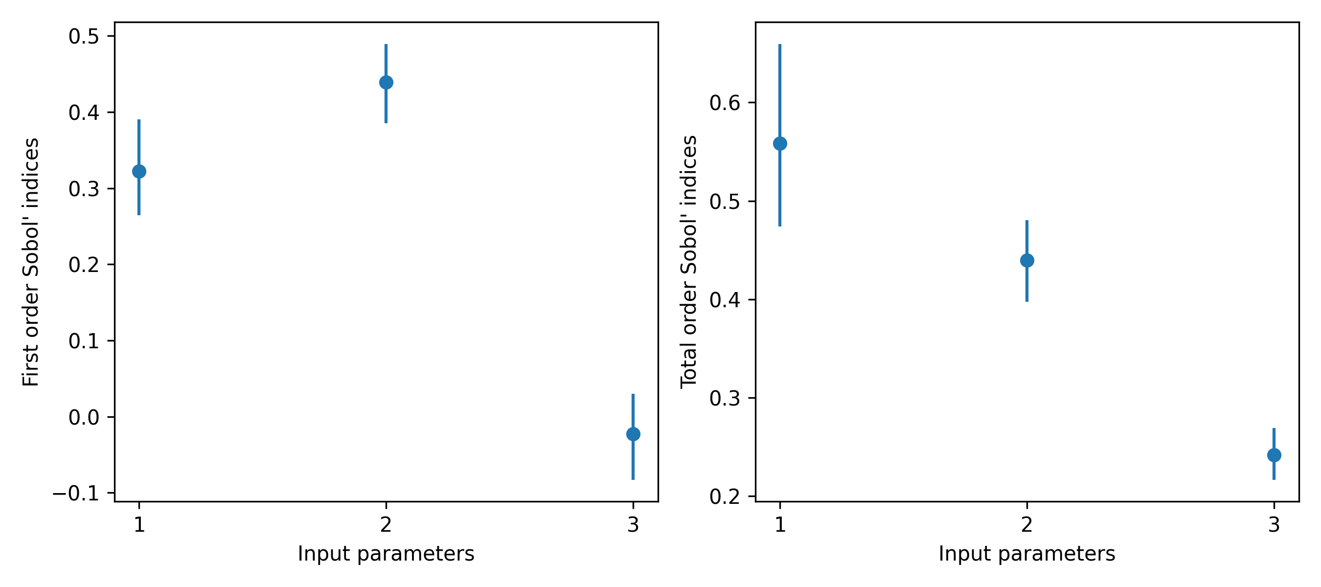
Then, this information can be easily visualized.

import matplotlib.pyplot as plt
fig, axs = plt.subplots(1, 2, figsize=(9, 4))
_ = axs[0].errorbar(
    [1, 2, 3], indices.first_order, fmt='o',
    yerr=[
        indices.first_order - boot.first_order.confidence_interval.low,
        boot.first_order.confidence_interval.high - indices.first_order
    ],
)

✓

axs[0].set_ylabel("First order Sobol' indices")
axs[0].set_xlabel('Input parameters')
axs[0].set_xticks([1, 2, 3])

✗

_ = axs[1].errorbar(
    [1, 2, 3], indices.total_order, fmt='o',
    yerr=[
        indices.total_order - boot.total_order.confidence_interval.low,
        boot.total_order.confidence_interval.high - indices.total_order
    ],
)

✓

axs[1].set_ylabel("Total order Sobol' indices")
axs[1].set_xlabel('Input parameters')
axs[1].set_xticks([1, 2, 3])

✗

plt.tight_layout()
plt.show()

✓

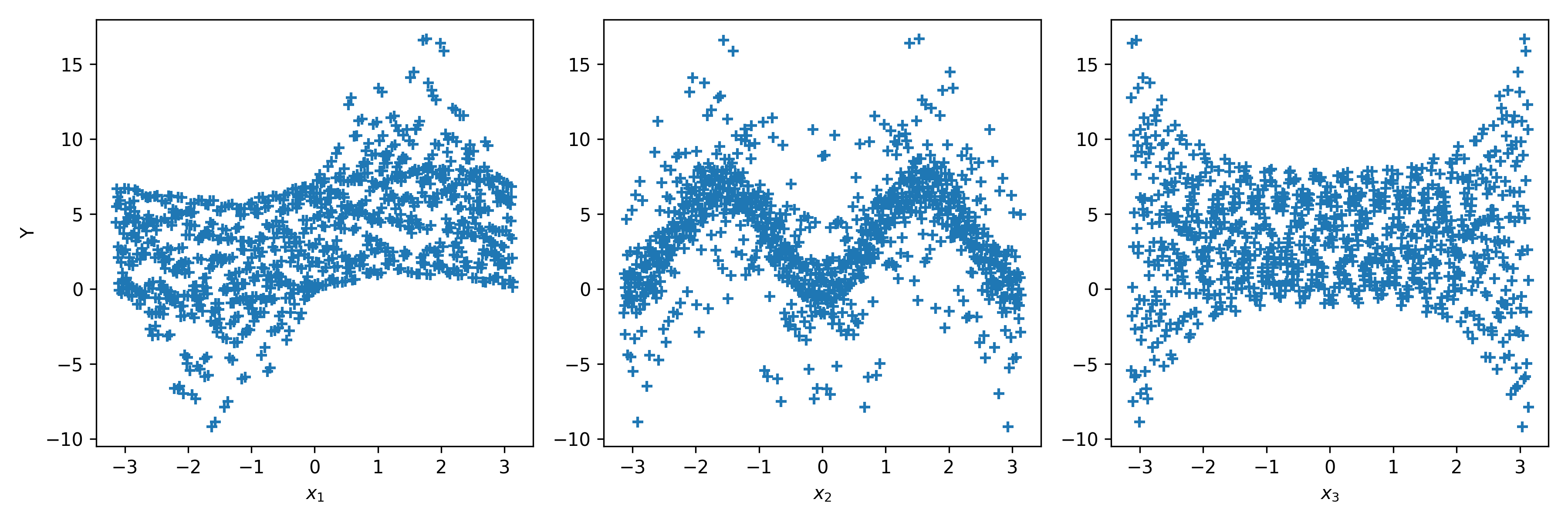
.. note:: By default, `scipy.stats.uniform` has support ``[0, 1]``. Using the parameters ``loc`` and ``scale``, one obtains the uniform distribution on ``[loc, loc + scale]``. This result is particularly interesting because the first order index :math:`S_{x_3} = 0` whereas its total order is :math:`S_{T_{x_3}} = 0.244`. This means that higher order interactions with :math:`x_3` are responsible for the difference. Almost 25% of the observed variance on the QoI is due to the correlations between :math:`x_3` and :math:`x_1`, although :math:`x_3` by itself has no impact on the QoI. The following gives a visual explanation of Sobol' indices on this function. Let's generate 1024 samples in :math:`[-\pi, \pi]^3` and calculate the value of the output.

from scipy.stats import qmc
n_dim = 3
p_labels = ['$x_1$', '$x_2$', '$x_3$']
sample = qmc.Sobol(d=n_dim, seed=rng).random(1024)
sample = qmc.scale(
    sample=sample,
    l_bounds=[-np.pi, -np.pi, -np.pi],
    u_bounds=[np.pi, np.pi, np.pi]
)
output = f_ishigami(sample.T)

✓

Now we can do scatter plots of the output with respect to each parameter. This gives a visual way to understand how each parameter impacts the output of the function.

fig, ax = plt.subplots(1, n_dim, figsize=(12, 4))

✓

for i in range(n_dim):
    xi = sample[:, i]
    ax[i].scatter(xi, output, marker='+')
    ax[i].set_xlabel(p_labels[i])
ax[0].set_ylabel('Y')

✗

plt.tight_layout()
plt.show()

✓

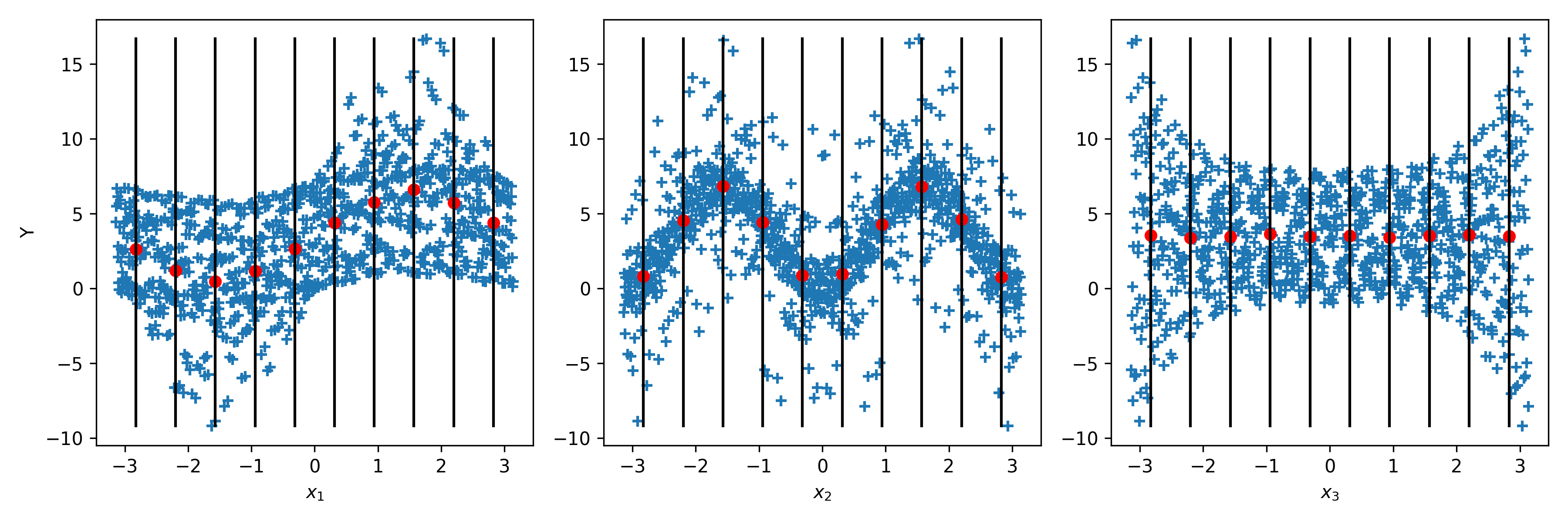
Now Sobol' goes a step further: by conditioning the output value by given values of the parameter (black lines), the conditional output mean is computed. It corresponds to the term :math:`\mathbb{E}(Y|x_i)`. Taking the variance of this term gives the numerator of the Sobol' indices.

mini = np.min(output)
maxi = np.max(output)
n_bins = 10
bins = np.linspace(-np.pi, np.pi, num=n_bins, endpoint=False)
dx = bins[1] - bins[0]
fig, ax = plt.subplots(1, n_dim, figsize=(12, 4))

✓

for i in range(n_dim):
    xi = sample[:, i]
    ax[i].scatter(xi, output, marker='+')
    ax[i].set_xlabel(p_labels[i])
    for bin_ in bins:
        idx = np.where((bin_ <= xi) & (xi <= bin_ + dx))
        xi_ = xi[idx]
        y_ = output[idx]
        ave_y_ = np.mean(y_)
        ax[i].plot([bin_ + dx/2] * 2, [mini, maxi], c='k')
        ax[i].scatter(bin_ + dx/2, ave_y_, c='r')
ax[0].set_ylabel('Y')

✗

plt.tight_layout()
plt.show()

✓

Looking at :math:`x_3`, the variance of the mean is zero leading to :math:`S_{x_3} = 0`. But we can further observe that the variance of the output is not constant along the parameter values of :math:`x_3`. This heteroscedasticity is explained by higher order interactions. Moreover, an heteroscedasticity is also noticeable on :math:`x_1` leading to an interaction between :math:`x_3` and :math:`x_1`. On :math:`x_2`, the variance seems to be constant and thus null interaction with this parameter can be supposed. This case is fairly simple to analyse visually---although it is only a qualitative analysis. Nevertheless, when the number of input parameters increases such analysis becomes unrealistic as it would be difficult to conclude on high-order terms. Hence the benefit of using Sobol' indices.

Aliases

scipy.stats.sobol_indices

`scipy.stats._sensitivity_analysis:sobol_indices`

Signature

Summary

Parameters

Returns

Notes

Examples

Aliases

Referenced by

This package