{ } Raw JSON

bundles / scipy latest / scipy / stats / _survival / ecdf

function

`scipy.stats._survival:ecdf`

source: /scipy/stats/_survival.py :253

Signature

def ecdf ( sample : npt.ArrayLike | CensoredData ) → ECDFResult

Summary

Empirical cumulative distribution function of a sample.

Extended Summary

The empirical cumulative distribution function (ECDF) is a step function estimate of the CDF of the distribution underlying a sample. This function returns objects representing both the empirical distribution function and its complement, the empirical survival function.

Parameters

sample : 1D array_like or `scipy.stats.CensoredData`: Besides array_like, instances of scipy.stats.CensoredData containing uncensored and right-censored observations are supported. Currently, other instances of scipy.stats.CensoredData will result in a NotImplementedError.

Returns

res : `~scipy.stats._result_classes.ECDFResult`

An object with the following attributes.

cdf: cdf
sf: sf

The cdf and sf attributes themselves have the following attributes.

quantiles: quantiles
probabilities: probabilities

And the following methods:

evaluate(x) :: Evaluate the CDF/SF at the argument.
plot(ax) :: Plot the CDF/SF on the provided axes.
confidence_interval(confidence_level=0.95) :: Compute the confidence interval around the CDF/SF at the values in quantiles.

Notes

When each observation of the sample is a precise measurement, the ECDF steps up by 1/len(sample) at each of the observations ^[1].

When observations are lower bounds, upper bounds, or both upper and lower bounds, the data is said to be "censored", and sample may be provided as an instance of scipy.stats.CensoredData.

For right-censored data, the ECDF is given by the Kaplan-Meier estimator ^[2]; other forms of censoring are not supported at this time.

Confidence intervals are computed according to the Greenwood formula or the more recent "Exponential Greenwood" formula as described in ^[4].

Array API Standard Support

ecdf has experimental support for Python Array API Standard compatible backends in addition to NumPy. Please consider testing these features by setting an environment variable SCIPY_ARRAY_API=1 and providing CuPy, PyTorch, JAX, or Dask arrays as array arguments. The following combinations of backend and device (or other capability) are supported.

====================  ====================  ====================
Library               CPU                   GPU
====================  ====================  ====================
NumPy                 ✅                     n/a                 
CuPy                  n/a                   ⛔                   
PyTorch               ⛔                     ⛔                   
JAX                   ⛔                     ⛔                   
Dask                  ⛔                     n/a                 
====================  ====================  ====================

See dev-arrayapi for more information.

Examples

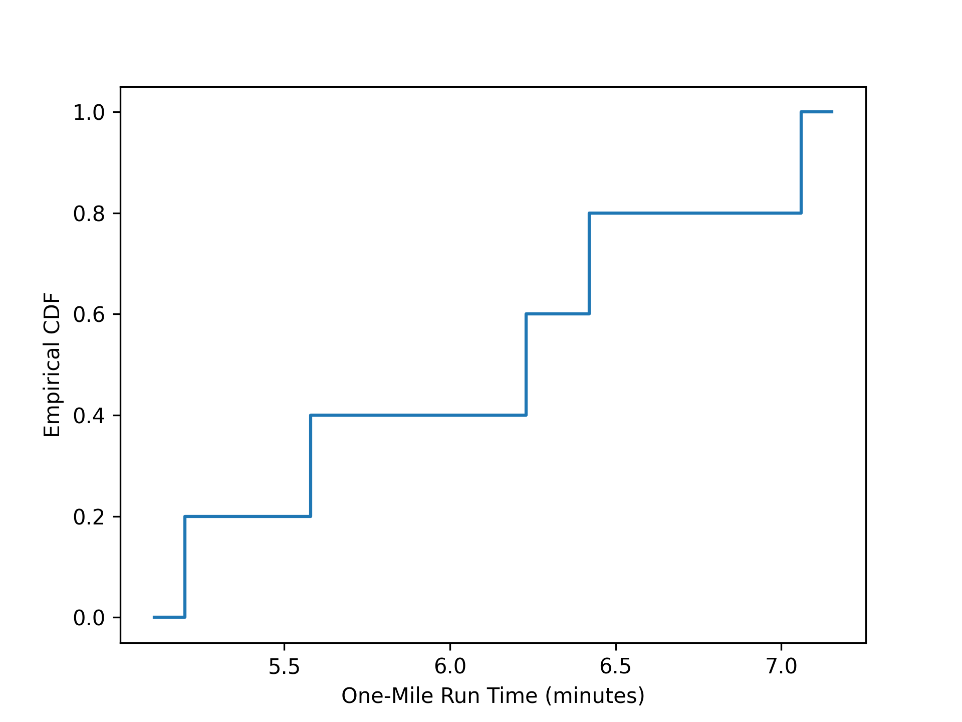
**Uncensored Data** As in the example from [1]_ page 79, five boys were selected at random from those in a single high school. Their one-mile run times were recorded as follows.

sample = [6.23, 5.58, 7.06, 6.42, 5.20]  # one-mile run times (minutes)

✓

The empirical distribution function, which approximates the distribution function of one-mile run times of the population from which the boys were sampled, is calculated as follows.

from scipy import stats
res = stats.ecdf(sample)
res.cdf.quantiles
res.cdf.probabilities

✓

To plot the result as a step function:

import matplotlib.pyplot as plt
ax = plt.subplot()

✓

res.cdf.plot(ax)
ax.set_xlabel('One-Mile Run Time (minutes)')
ax.set_ylabel('Empirical CDF')

✗

plt.show()

✓

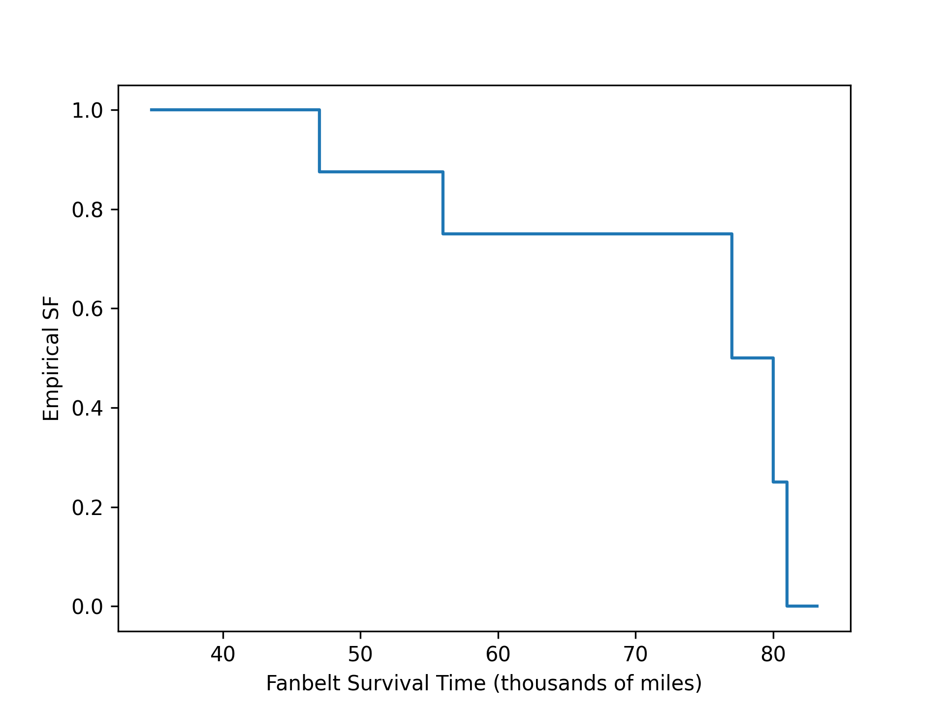
**Right-censored Data** As in the example from [1]_ page 91, the lives of ten car fanbelts were tested. Five tests concluded because the fanbelt being tested broke, but the remaining tests concluded for other reasons (e.g. the study ran out of funding, but the fanbelt was still functional). The mileage driven with the fanbelts were recorded as follows.

broken = [77, 47, 81, 56, 80]  # in thousands of miles driven
unbroken = [62, 60, 43, 71, 37]

✓

Precise survival times of the fanbelts that were still functional at the end of the tests are unknown, but they are known to exceed the values recorded in ``unbroken``. Therefore, these observations are said to be "right-censored", and the data is represented using `scipy.stats.CensoredData`.

sample = stats.CensoredData(uncensored=broken, right=unbroken)

✓

The empirical survival function is calculated as follows.

res = stats.ecdf(sample)
res.sf.quantiles

✓

res.sf.probabilities

✗