bundles / scipy latest / scipy / stats / _survival / logrank

function

`scipy.stats._survival:logrank`

source: /scipy/stats/_survival.py :488

Signature

   def     logrank (    x  :  npt.ArrayLike | CensoredData    ,    y  :  npt.ArrayLike | CensoredData    ,    alternative  :  Literal['two-sided', 'less', 'greater']    =  two-sided     )   →  LogRankResult

Summary

Compare the survival distributions of two samples via the logrank test.

Parameters

x, y : array_like or CensoredData

Samples to compare based on their empirical survival functions.

alternative : {'two-sided', 'less', 'greater'}, optional

Defines the alternative hypothesis.

The null hypothesis is that the survival distributions of the two groups, say X and Y, are identical.

The following alternative hypotheses ^[4] are available (default is 'two-sided'):

'two-sided': the survival distributions of the two groups are not identical.
'less': survival of group X is favored: the group X failure rate function is less than the group Y failure rate function at some times.
'greater': survival of group Y is favored: the group X failure rate function is greater than the group Y failure rate function at some times.

Returns

res : `~scipy.stats._result_classes.LogRankResult`

An object containing attributes:

statistic: statistic
pvalue: pvalue

Notes

The logrank test ^[1] compares the observed number of events to the expected number of events under the null hypothesis that the two samples were drawn from the same distribution. The statistic is

Z_{i} = \frac{\sum _{j = 1}^{J} ( O _{i, j} - E _{i, j} )}{\sum _{j = 1}^{J} V _{i, j}} \to N (0, 1)

where

E_{i, j} = O_{j} \frac{N _{i, j}}{N _{j}}, V_{i, j} = E_{i, j} (\frac{N _{j} - O _{j}}{N _{j}}) (\frac{N _{j} - N _{i, j}}{N _{j} - 1}),

$i$ denotes the group (i.e. it may assume values $x$ or $y$ , or it may be omitted to refer to the combined sample) $j$ denotes the time (at which an event occurred), $N$ is the number of subjects at risk just before an event occurred, and $O$ is the observed number of events at that time.

The statistic $Z_{x}$ returned by logrank is the (signed) square root of the statistic returned by many other implementations. Under the null hypothesis, $Z_{x} * * 2$ is asymptotically distributed according to the chi-squared distribution with one degree of freedom. Consequently, $Z_{x}$ is asymptotically distributed according to the standard normal distribution. The advantage of using $Z_{x}$ is that the sign information (i.e. whether the observed number of events tends to be less than or greater than the number expected under the null hypothesis) is preserved, allowing scipy.stats.logrank to offer one-sided alternative hypotheses.

Array API Standard Support

logrank has experimental support for Python Array API Standard compatible backends in addition to NumPy. Please consider testing these features by setting an environment variable SCIPY_ARRAY_API=1 and providing CuPy, PyTorch, JAX, or Dask arrays as array arguments. The following combinations of backend and device (or other capability) are supported.

====================  ====================  ====================
Library               CPU                   GPU
====================  ====================  ====================
NumPy                 ✅                     n/a                 
CuPy                  n/a                   ⛔                   
PyTorch               ⛔                     ⛔                   
JAX                   ⛔                     ⛔                   
Dask                  ⛔                     n/a                 
====================  ====================  ====================

See dev-arrayapi for more information.

Examples

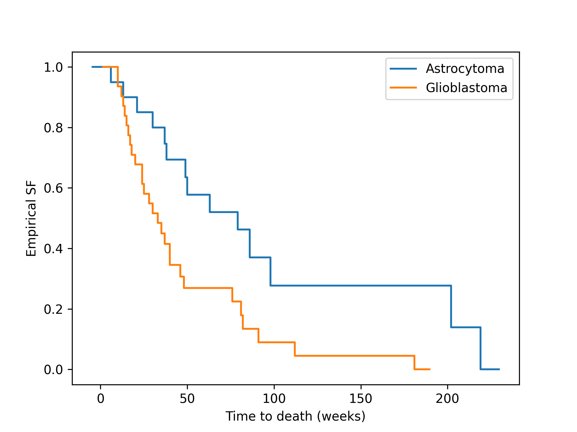
Reference [2]_ compared the survival times of patients with two different types of recurrent malignant gliomas. The samples below record the time (number of weeks) for which each patient participated in the study. The `scipy.stats.CensoredData` class is used because the data is right-censored: the uncensored observations correspond with observed deaths whereas the censored observations correspond with the patient leaving the study for another reason.

from scipy import stats
x = stats.CensoredData(
    uncensored=[6, 13, 21, 30, 37, 38, 49, 50,
                63, 79, 86, 98, 202, 219],
    right=[31, 47, 80, 82, 82, 149]
)
y = stats.CensoredData(
    uncensored=[10, 10, 12, 13, 14, 15, 16, 17, 18, 20, 24, 24,
                25, 28,30, 33, 35, 37, 40, 40, 46, 48, 76, 81,
                82, 91, 112, 181],
    right=[34, 40, 70]
)

✓

We can calculate and visualize the empirical survival functions of both groups as follows.

import numpy as np
import matplotlib.pyplot as plt
ax = plt.subplot()
ecdf_x = stats.ecdf(x)

✓

ecdf_x.sf.plot(ax, label='Astrocytoma')

✗

ecdf_y = stats.ecdf(y)

✓

ecdf_y.sf.plot(ax, label='Glioblastoma')
ax.set_xlabel('Time to death (weeks)')
ax.set_ylabel('Empirical SF')
plt.legend()

✗

plt.show()

✓

Visual inspection of the empirical survival functions suggests that the survival times tend to be different between the two groups. To formally assess whether the difference is significant at the 1% level, we use the logrank test.

res = stats.logrank(x=x, y=y)

✓

res.statistic
res.pvalue

✗

The p-value is less than 1%, so we can consider the data to be evidence against the null hypothesis in favor of the alternative that there is a difference between the two survival functions.

Aliases

scipy.stats.logrank