`scipy.signal._filter_design:bilinear`

source: /scipy/signal/_filter_design.py :2336

Signature

def bilinear ( b , a , fs = 1.0 )

Summary

Calculate a digital IIR filter from an analog transfer function by utilizing the bilinear transform.

Parameters

b : array_like: Coefficients of the numerator polynomial of the analog transfer function in form of a complex- or real-valued 1d array.
a : array_like: Coefficients of the denominator polynomial of the analog transfer function in form of a complex- or real-valued 1d array.
fs : float: Sample rate, as ordinary frequency (e.g., hertz). No pre-warping is done in this function.

Returns

beta : ndarray: Coefficients of the numerator polynomial of the digital transfer function in form of a complex- or real-valued 1d array.
alpha : ndarray: Coefficients of the denominator polynomial of the digital transfer function in form of a complex- or real-valued 1d array.

Notes

The parameters $b = [b_{0}, \dots, b_{Q}]$ and $a = [a_{0}, \dots, a_{P}]$ are 1d arrays of length $Q + 1$ and $P + 1$ . They define the analog transfer function

H_{a} (s) = \frac{b _{0} s ^{Q} + b _{1} s ^{Q - 1} + \dots + b _{Q}}{a _{0} s ^{P} + a _{1} s ^{P - 1} + \dots + a _{P}} .

The bilinear transform ^[1] is applied by substituting

s = κ \frac{z - 1}{z + 1}, κ := 2 f_{s},

into $H_{a} (s)$ , with $f_{s}$ being the sampling rate. This results in the digital transfer function in the $z$ -domain

H_{d} (z) = \frac{b _{0} ( κ \frac{z - 1}{z + 1} ) ^{Q} + b _{1} ( κ \frac{z - 1}{z + 1} ) ^{Q - 1} + \dots + b _{Q}}{a _{0} ( κ \frac{z - 1}{z + 1} ) ^{P} + a _{1} ( κ \frac{z - 1}{z + 1} ) ^{P - 1} + \dots + a _{P}} .

This expression can be simplified by multiplying numerator and denominator by $(z + 1)^{N}$ , with $N = max (P, Q)$ . This allows $H_{d} (z)$ to be reformulated as

=: \frac{b _{0} ( κ ( z - 1 ) ) ^{Q} ( z + 1 ) ^{N - Q} + b _{1} ( κ ( z - 1 ) ) ^{Q - 1} ( z + 1 ) ^{N - Q + 1} + \dots + b _{Q} ( z + 1 ) ^{N}}{a _{0} ( κ ( z - 1 ) ) ^{P} ( z + 1 ) ^{N - P} + a _{1} ( κ ( z - 1 ) ) ^{P - 1} ( z + 1 ) ^{N - P + 1} + \dots + a _{P} ( z + 1 ) ^{N}} \frac{β _{0} + β _{1} z ^{- 1} + \dots + β _{N} z ^{- N}}{α _{0} + α _{1} z ^{- 1} + \dots + α _{N} z ^{- N}} .

This is the equation implemented to perform the bilinear transform. Note that for large $f_{s}$ , $κ^{Q}$ or $κ^{P}$ can cause a numeric overflow for sufficiently large $P$ or $Q$ .

Array API Standard Support

bilinear has experimental support for Python Array API Standard compatible backends in addition to NumPy. Please consider testing these features by setting an environment variable SCIPY_ARRAY_API=1 and providing CuPy, PyTorch, JAX, or Dask arrays as array arguments. The following combinations of backend and device (or other capability) are supported.

====================  ====================  ====================
Library               CPU                   GPU
====================  ====================  ====================
NumPy                 ✅                     n/a                 
CuPy                  n/a                   ✅                   
PyTorch               ✅                     ⛔                   
JAX                   ⚠️ no JIT             ⛔                   
Dask                  ⚠️ computes graph     n/a                 
====================  ====================  ====================

CuPy does not accept complex inputs.

See dev-arrayapi for more information.

Examples

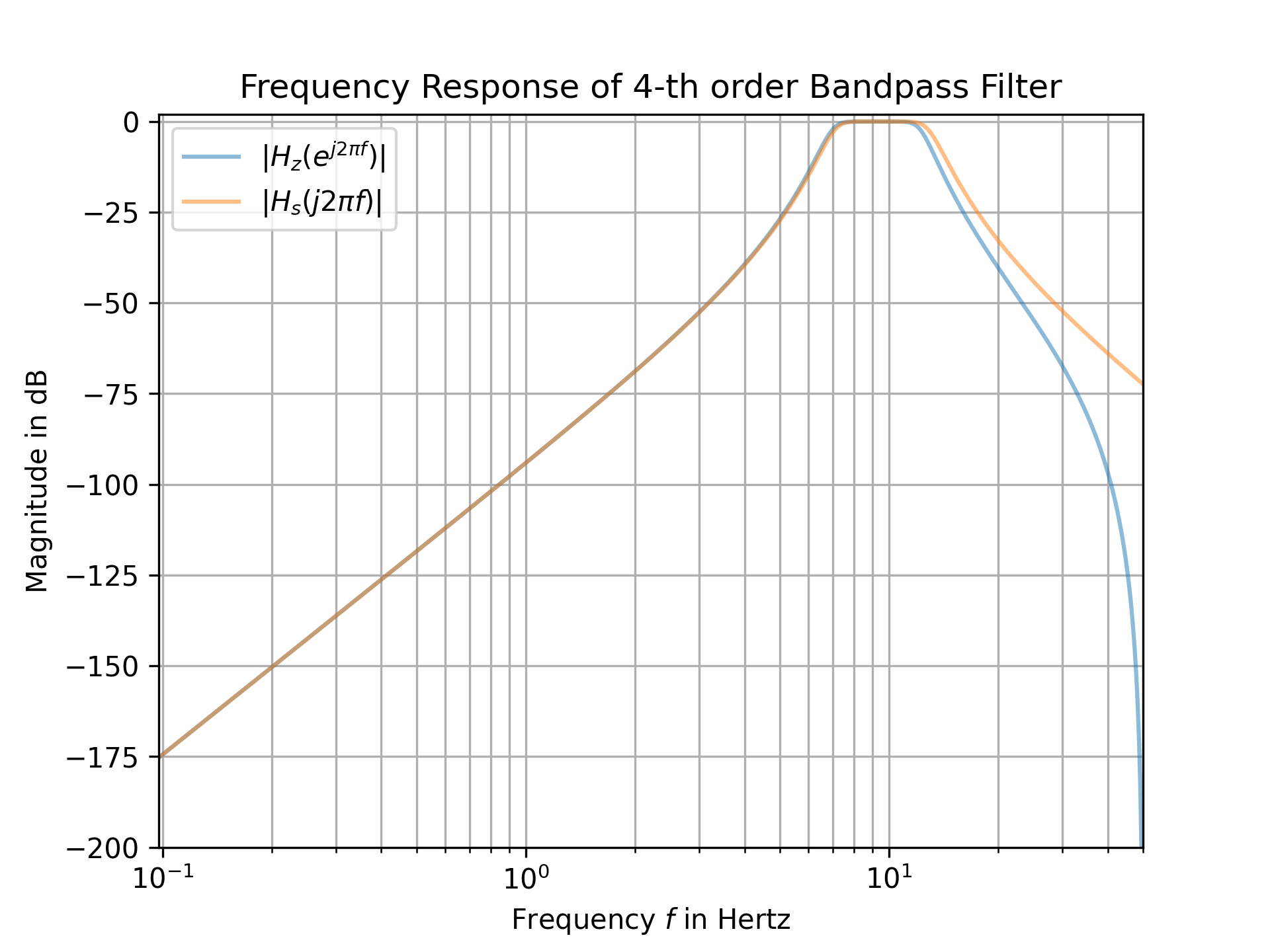
The following example shows the frequency response of an analog bandpass filter and the corresponding digital filter derived by utilitzing the bilinear transform:

from scipy import signal
import matplotlib.pyplot as plt
import numpy as np
fs = 100  # sampling frequency
om_c = 2 * np.pi * np.array([7, 13])  # corner frequencies
bb_s, aa_s = signal.butter(4, om_c, btype='bandpass', analog=True, output='ba')
bb_z, aa_z = signal.bilinear(bb_s, aa_s, fs)
w_z, H_z = signal.freqz(bb_z, aa_z)  # frequency response of digitial filter
w_s, H_s = signal.freqs(bb_s, aa_s, worN=w_z*fs)  # analog filter response
f_z, f_s = w_z * fs / (2*np.pi), w_s / (2*np.pi)
Hz_dB, Hs_dB = (20*np.log10(np.abs(H_).clip(1e-10)) for H_ in (H_z, H_s))
fg0, ax0 = plt.subplots()

✓

ax0.set_title("Frequency Response of 4-th order Bandpass Filter")
ax0.set(xlabel='Frequency $f$ in Hertz', ylabel='Magnitude in dB',
        xlim=[f_z[1], fs/2], ylim=[-200, 2])
ax0.semilogx(f_z, Hz_dB, alpha=.5, label=r'$|H_z(e^{j 2 \pi f})|$')
ax0.semilogx(f_s, Hs_dB, alpha=.5, label=r'$|H_s(j 2 \pi f)|$')
ax0.legend()

✗

ax0.grid(which='both', axis='x')
ax0.grid(which='major', axis='y')
plt.show()

✓

The difference in the higher frequencies shown in the plot is caused by an effect called "frequency warping". [1]_ describes a method called "pre-warping" to reduce those deviations.

`scipy.signal._filter_design:bilinear`

Signature

Summary

Parameters

Returns

Notes

Examples

See also

Aliases

Referenced by

This package