bundles / scipy 1.17.1 / scipy / signal / _spectral_py / spectrogram
function
scipy.signal._spectral_py:spectrogram
Signature
def spectrogram ( x , fs = 1.0 , window = ('tukey_periodic', 0.25) , nperseg = None , noverlap = None , nfft = None , detrend = constant , return_onesided = True , scaling = density , axis = -1 , mode = psd ) Summary
Compute a spectrogram with consecutive Fourier transforms (legacy function).
Extended Summary
Spectrograms can be used as a way of visualizing the change of a nonstationary signal's frequency content over time.
Parameters
x: array_likeTime series of measurement values
fs: float, optionalSampling frequency of the
xtime series. Defaults to 1.0.window: str or tuple or array_like, optionalDesired window to use. If
windowis a string or tuple, it is passed to get_window to generate the window values, which are DFT-even by default. See get_window for a list of windows and required parameters. Ifwindowis array_like it will be used directly as the window and its length must be nperseg. Defaults to a periodic Tukey window with shape parameter of 0.25.nperseg: int, optionalLength of each segment. Defaults to None, but if window is str or tuple, is set to 256, and if window is array_like, is set to the length of the window.
noverlap: int, optionalNumber of points to overlap between segments. If
None,noverlap = nperseg // 8. Defaults toNone.nfft: int, optionalLength of the FFT used, if a zero padded FFT is desired. If
None, the FFT length isnperseg. Defaults toNone.detrend: str or function or `False`, optionalSpecifies how to detrend each segment. If
detrendis a string, it is passed as thetypeargument to thedetrendfunction. If it is a function, it takes a segment and returns a detrended segment. IfdetrendisFalse, no detrending is done. Defaults to 'constant'.return_onesided: bool, optionalIf
True, return a one-sided spectrum for real data. IfFalsereturn a two-sided spectrum. Defaults toTrue, but for complex data, a two-sided spectrum is always returned.scaling: { 'density', 'spectrum' }, optionalSelects between computing the power spectral density ('density') where Sxx has units of V**2/Hz and computing the power spectrum ('spectrum') where Sxx has units of V**2, if
xis measured in V andfsis measured in Hz. Defaults to 'density'.axis: int, optionalAxis along which the spectrogram is computed; the default is over the last axis (i.e.
axis=-1).mode: str, optionalDefines what kind of return values are expected. Options are ['psd', 'complex', 'magnitude', 'angle', 'phase']. 'complex' is equivalent to the output of
stftwith no padding or boundary extension. 'magnitude' returns the absolute magnitude of the STFT. 'angle' and 'phase' return the complex angle of the STFT, with and without unwrapping, respectively.
Returns
f: ndarrayArray of sample frequencies.
t: ndarrayArray of segment times.
Sxx: ndarraySpectrogram of x. By default, the last axis of Sxx corresponds to the segment times.
Notes
An appropriate amount of overlap will depend on the choice of window and on your requirements. In contrast to welch's method, where the entire data stream is averaged over, one may wish to use a smaller overlap (or perhaps none at all) when computing a spectrogram, to maintain some statistical independence between individual segments. It is for this reason that the default window is a Tukey window with 1/8th of a window's length overlap at each end.
Array API Standard Support
spectrogram is not in-scope for support of Python Array API Standard compatible backends other than NumPy.
See dev-arrayapi for more information.
Examples
import numpy as np
from scipy import signal
from scipy.fft import fftshift
import matplotlib.pyplot as plt
rng = np.random.default_rng()
✓
fs = 10e3
N = 1e5
amp = 2 * np.sqrt(2)
noise_power = 0.01 * fs / 2
time = np.arange(N) / float(fs)
mod = 500*np.cos(2*np.pi*0.25*time)
carrier = amp * np.sin(2*np.pi*3e3*time + mod)
noise = rng.normal(scale=np.sqrt(noise_power), size=time.shape)
noise *= np.exp(-time/5)
x = carrier + noise
✓
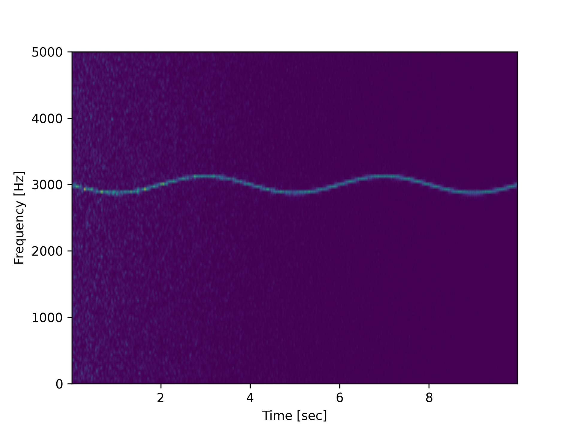
f, t, Sxx = signal.spectrogram(x, fs)
✓plt.pcolormesh(t, f, Sxx, shading='gouraud') plt.ylabel('Frequency [Hz]') plt.xlabel('Time [sec]')✗
plt.show()
✓
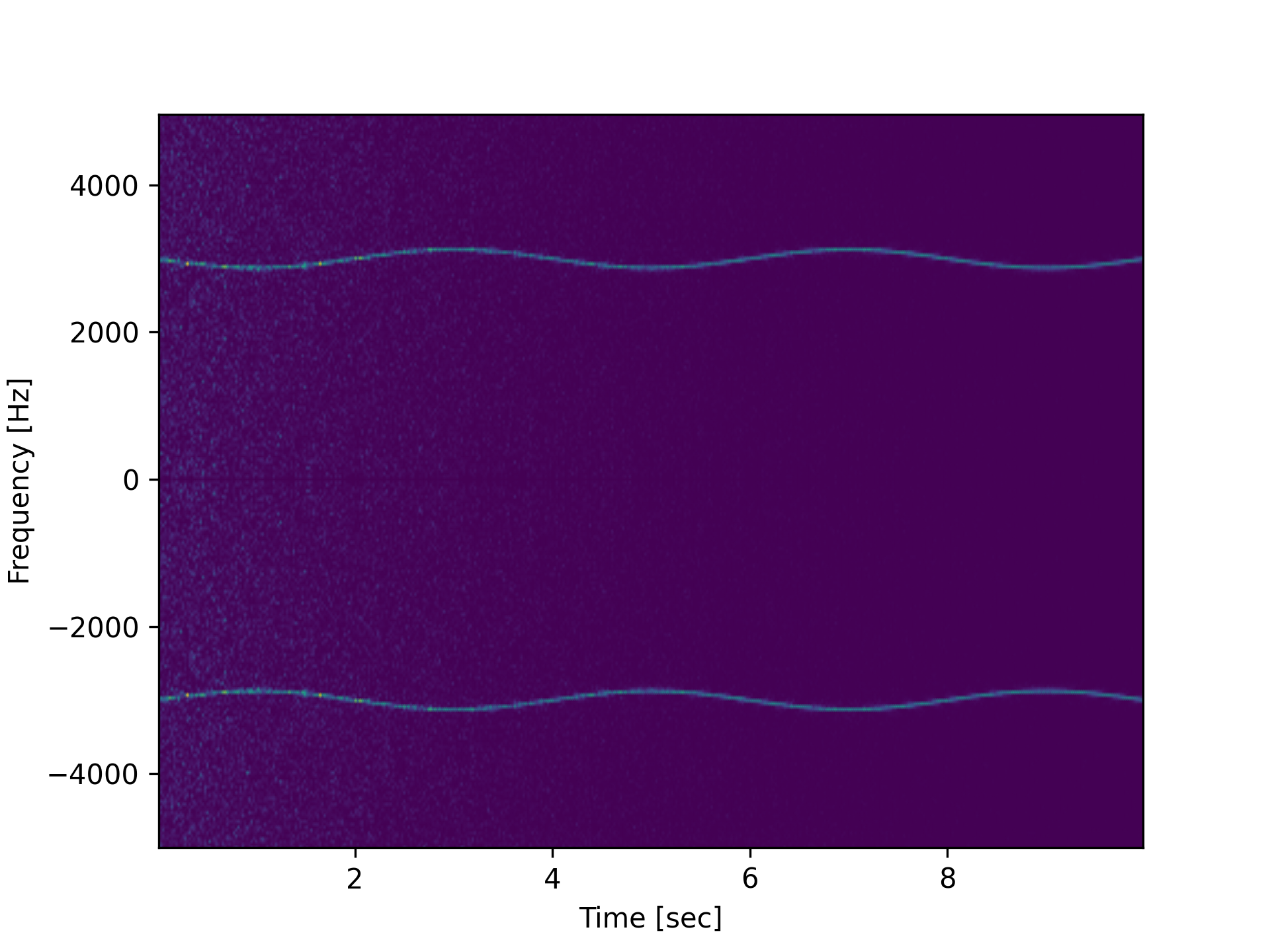
f, t, Sxx = signal.spectrogram(x, fs, return_onesided=False)
✓plt.pcolormesh(t, fftshift(f), fftshift(Sxx, axes=0), shading='gouraud') plt.ylabel('Frequency [Hz]') plt.xlabel('Time [sec]')✗
plt.show()
✓
See also
- ShortTimeFFT
Newer STFT/ISTFT implementation providing more features, which also includes a
~ShortTimeFFT.spectrogrammethod.- csd
Cross spectral density by Welch's method.
- lombscargle
Lomb-Scargle periodogram for unevenly sampled data
- periodogram
Simple, optionally modified periodogram
- welch
Power spectral density by Welch's method.
Aliases
-
scipy.signal.spectrogram