`scipy.signal._ltisys:dimpulse`

source: build-install/usr/lib/python3.14/site-packages/scipy/signal/_ltisys.py:3463

Signature

def dimpulse(system, x0 = None, t = None, n = None)

Summary

Impulse response of discrete-time system.

Parameters

system : dlti | tuple

An instance of the LTI class dlti or a tuple describing the system. The number of elements in the tuple determine the interpretation. I.e.:

system: Instance of LTI class dlti. Note that derived instances, such as instances of TransferFunction, ZerosPolesGain, or StateSpace, are allowed as well.
(num, den, dt): Rational polynomial as described in TransferFunction. The coefficients of the polynomials should be specified in descending exponent order, e.g., z² + 3z + 5 would be represented as [1, 3, 5].
(zeros, poles, gain, dt): Zeros, poles, gain form as described in ZerosPolesGain.
(A, B, C, D, dt): State-space form as described in StateSpace.

x0 : array_like, optional

Initial state-vector. Defaults to zero.

t : array_like, optional

Time points. Computed if not given.

n : int, optional

The number of time points to compute (if t is not given).

Returns

tout : ndarray: Time values for the output, as a 1-D array.
yout : tuple of ndarray: Impulse response of system. Each element of the tuple represents the output of the system based on an impulse in each input.

Examples

import numpy as np
from scipy import signal
import matplotlib.pyplot as plt
dt = 1  # sampling interval is one => time unit is sample number
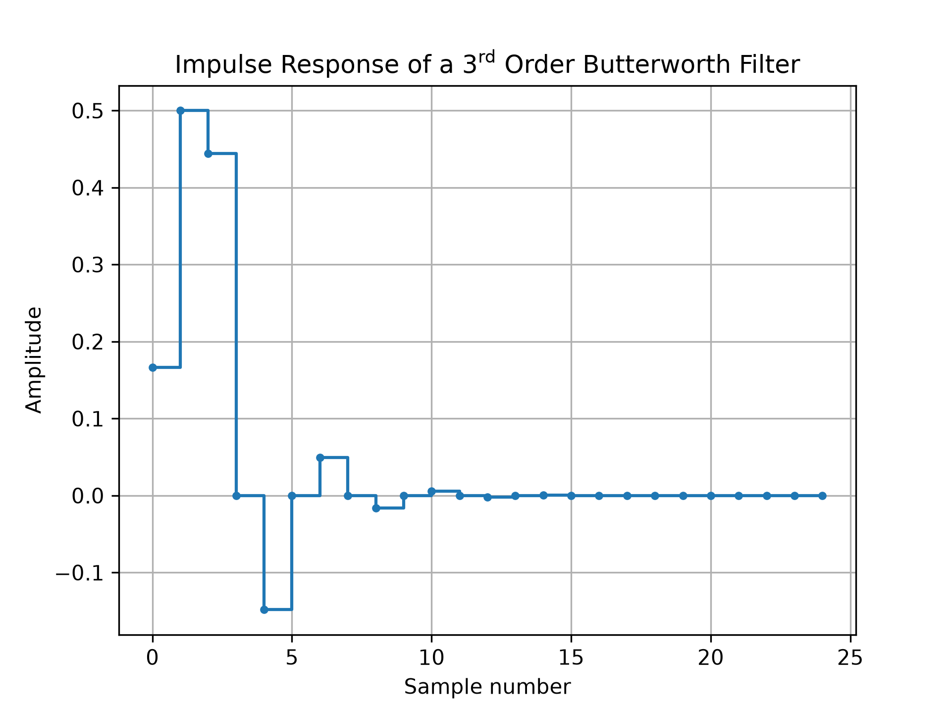
bb, aa = signal.butter(3, 0.25, fs=1/dt)
t, y = signal.dimpulse((bb, aa, dt), n=25)
fig0, ax0 = plt.subplots()

✓

ax0.step(t, np.squeeze(y), '.-', where='post')
ax0.set_title(r"Impulse Response of a $3^\text{rd}$ Order Butterworth Filter")
ax0.set(xlabel='Sample number', ylabel='Amplitude')

✗

[Text(0.5, 0, 'Sample number'), Text(0, 0.5, 'Amplitude')]

ax0.grid()
plt.show()

✓

Aliases

scipy.signal.dimpulse