`scipy.stats._morestats:probplot`

source: build-install/usr/lib/python3.14/site-packages/scipy/stats/_morestats.py:536

Signature

def probplot(x, sparams = (), dist = norm, fit = True, plot = None, rvalue = False)

Summary

Calculate quantiles for a probability plot, and optionally show the plot.

Extended Summary

Generates a probability plot of sample data against the quantiles of a specified theoretical distribution (the normal distribution by default). probplot optionally calculates a best-fit line for the data and plots the results using Matplotlib or a given plot function.

Parameters

x : array_like: Sample/response data from which probplot creates the plot.
sparams : tuple, optional: Distribution-specific shape parameters (shape parameters plus location and scale).
dist : str or stats.distributions instance, optional: Distribution or distribution function name. The default is 'norm' for a normal probability plot. Objects that look enough like a stats.distributions instance (i.e. they have a ppf method) are also accepted.
fit : bool, optional: Fit a least-squares regression (best-fit) line to the sample data if True (default).
plot : object, optional: If given, plots the quantiles. If given and fit is True, also plots the least squares fit. plot is an object that has to have methods "plot" and "text". The matplotlib.pyplot module or a Matplotlib Axes object can be used, or a custom object with the same methods. Default is None, which means that no plot is created.
rvalue : bool, optional: If plot is provided and fit is True, setting rvalue to True includes the coefficient of determination on the plot. Default is False.

Returns

(osm, osr) : tuple of ndarrays: Tuple of theoretical quantiles (osm, or order statistic medians) and ordered responses (osr). osr is simply sorted input x. For details on how osm is calculated see the Notes section.
(slope, intercept, r) : tuple of floats, optional: Tuple containing the result of the least-squares fit, if that is performed by probplot. r is the square root of the coefficient of determination. If fit=False and plot=None, this tuple is not returned.

Notes

Even if plot is given, the figure is not shown or saved by probplot; plt.show() or plt.savefig('figname.png') should be used after calling probplot.

probplot generates a probability plot, which should not be confused with a Q-Q or a P-P plot. Statsmodels has more extensive functionality of this type, see statsmodels.api.ProbPlot.

The formula used for the theoretical quantiles (horizontal axis of the probability plot) is Filliben's estimate

quantiles = dist.ppf(val), for

        0.5**(1/n),                  for i = n
  val = (i - 0.3175) / (n + 0.365),  for i = 2, ..., n-1
        1 - 0.5**(1/n),              for i = 1

where i indicates the i-th ordered value and n is the total number of values.

Examples

import numpy as np
from scipy import stats
import matplotlib.pyplot as plt
nsample = 100
rng = np.random.default_rng()

✓

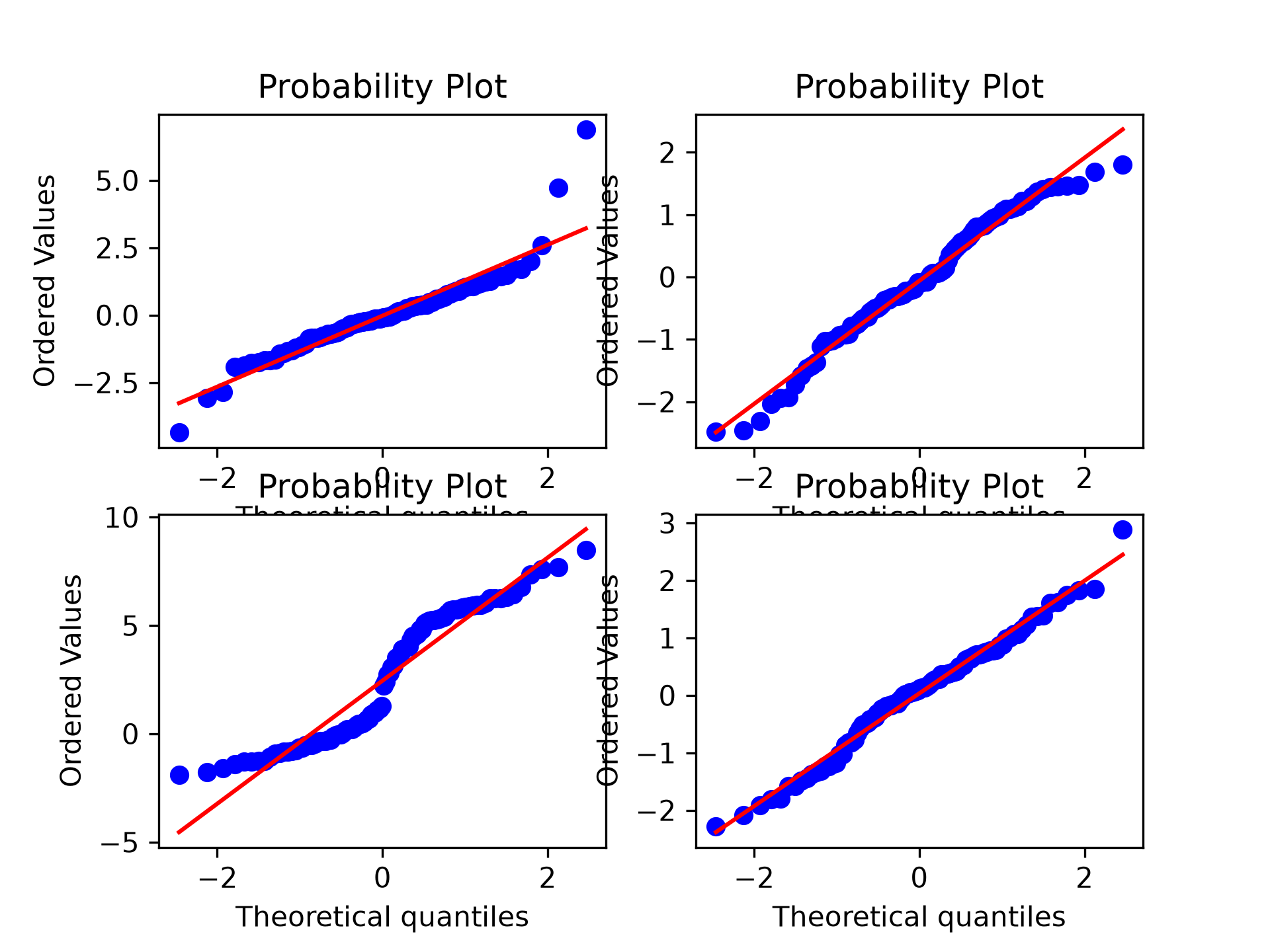
A t distribution with small degrees of freedom:

ax1 = plt.subplot(221)
x = stats.t.rvs(3, size=nsample, random_state=rng)
res = stats.probplot(x, plot=plt)

✓

A t distribution with larger degrees of freedom:

ax2 = plt.subplot(222)
x = stats.t.rvs(25, size=nsample, random_state=rng)
res = stats.probplot(x, plot=plt)

✓

A mixture of two normal distributions with broadcasting:

ax3 = plt.subplot(223)
x = stats.norm.rvs(loc=[0,5], scale=[1,1.5],
                   size=(nsample//2,2), random_state=rng).ravel()
res = stats.probplot(x, plot=plt)

✓

A standard normal distribution:

ax4 = plt.subplot(224)
x = stats.norm.rvs(loc=0, scale=1, size=nsample, random_state=rng)
res = stats.probplot(x, plot=plt)

✓

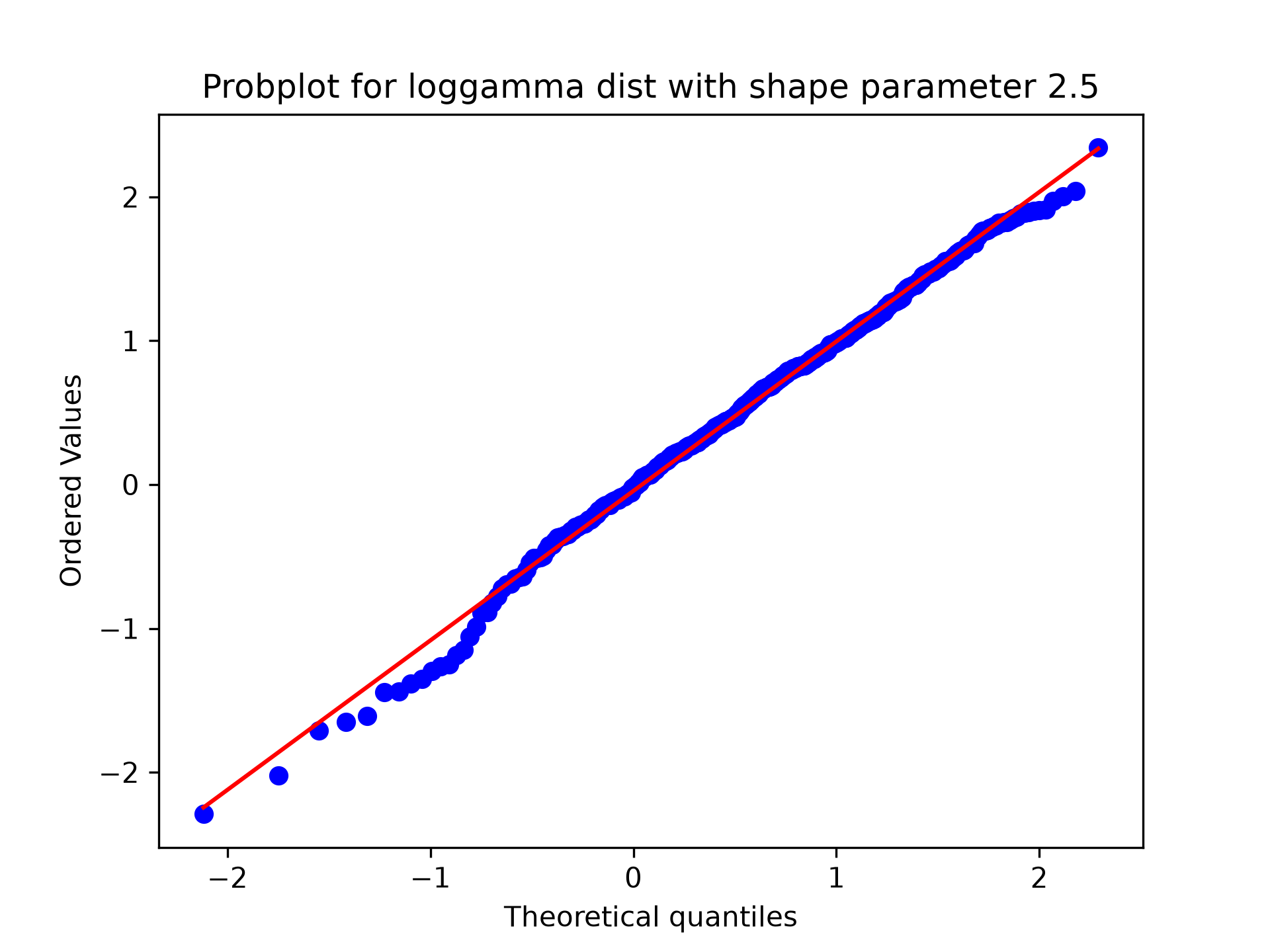
Produce a new figure with a loggamma distribution, using the ``dist`` and ``sparams`` keywords:

fig = plt.figure()
ax = fig.add_subplot(111)
x = stats.loggamma.rvs(c=2.5, size=500, random_state=rng)
res = stats.probplot(x, dist=stats.loggamma, sparams=(2.5,), plot=ax)

✓

ax.set_title("Probplot for loggamma dist with shape parameter 2.5")

✗

Text(0.5, 1.0, 'Probplot for loggamma dist with shape parameter 2.5')

Show the results with Matplotlib:

plt.show()

✓

Aliases

scipy.stats.probplot