`scipy.signal._ltisys:dfreqresp`

source: /scipy/signal/_ltisys.py :3349

Signature

def dfreqresp ( system , w = None , n = 10000 , whole = False )

Summary

Calculate the frequency response of a discrete-time system.

Parameters

system : dlti | tuple

An instance of the LTI class dlti or a tuple describing the system. The number of elements in the tuple determine the interpretation. I.e.:

system: Instance of LTI class dlti. Note that derived instances, such as instances of TransferFunction, ZerosPolesGain, or StateSpace, are allowed as well.
(num, den, dt): Rational polynomial as described in TransferFunction. The coefficients of the polynomials should be specified in descending exponent order, e.g., z² + 3z + 5 would be represented as [1, 3, 5].
(zeros, poles, gain, dt): Zeros, poles, gain form as described in ZerosPolesGain.
(A, B, C, D, dt): State-space form as described in StateSpace.

w : array_like, optional

Array of frequencies (in radians/sample). Magnitude and phase data is calculated for every value in this array. If not given a reasonable set will be calculated.

n : int, optional

Number of frequency points to compute if w is not given. The n frequencies are logarithmically spaced in an interval chosen to include the influence of the poles and zeros of the system.

whole : bool, optional

Normally, if 'w' is not given, frequencies are computed from 0 to the Nyquist frequency, pi radians/sample (upper-half of unit-circle). If whole is True, compute frequencies from 0 to 2*pi radians/sample.

Returns

w : 1D ndarray: Frequency array [radians/sample]
H : 1D ndarray: Array of complex magnitude values

Notes

If (num, den) is passed in for system, coefficients for both the numerator and denominator should be specified in descending exponent order (e.g. z^2 + 3z + 5 would be represented as [1, 3, 5]).

Array API Standard Support

dfreqresp has experimental support for Python Array API Standard compatible backends in addition to NumPy. Please consider testing these features by setting an environment variable SCIPY_ARRAY_API=1 and providing CuPy, PyTorch, JAX, or Dask arrays as array arguments. The following combinations of backend and device (or other capability) are supported.

====================  ====================  ====================
Library               CPU                   GPU
====================  ====================  ====================
NumPy                 ✅                     n/a                 
CuPy                  n/a                   ⛔                   
PyTorch               ⛔                     ⛔                   
JAX                   ⛔                     ⛔                   
Dask                  ⛔                     n/a                 
====================  ====================  ====================

See dev-arrayapi for more information.

Examples

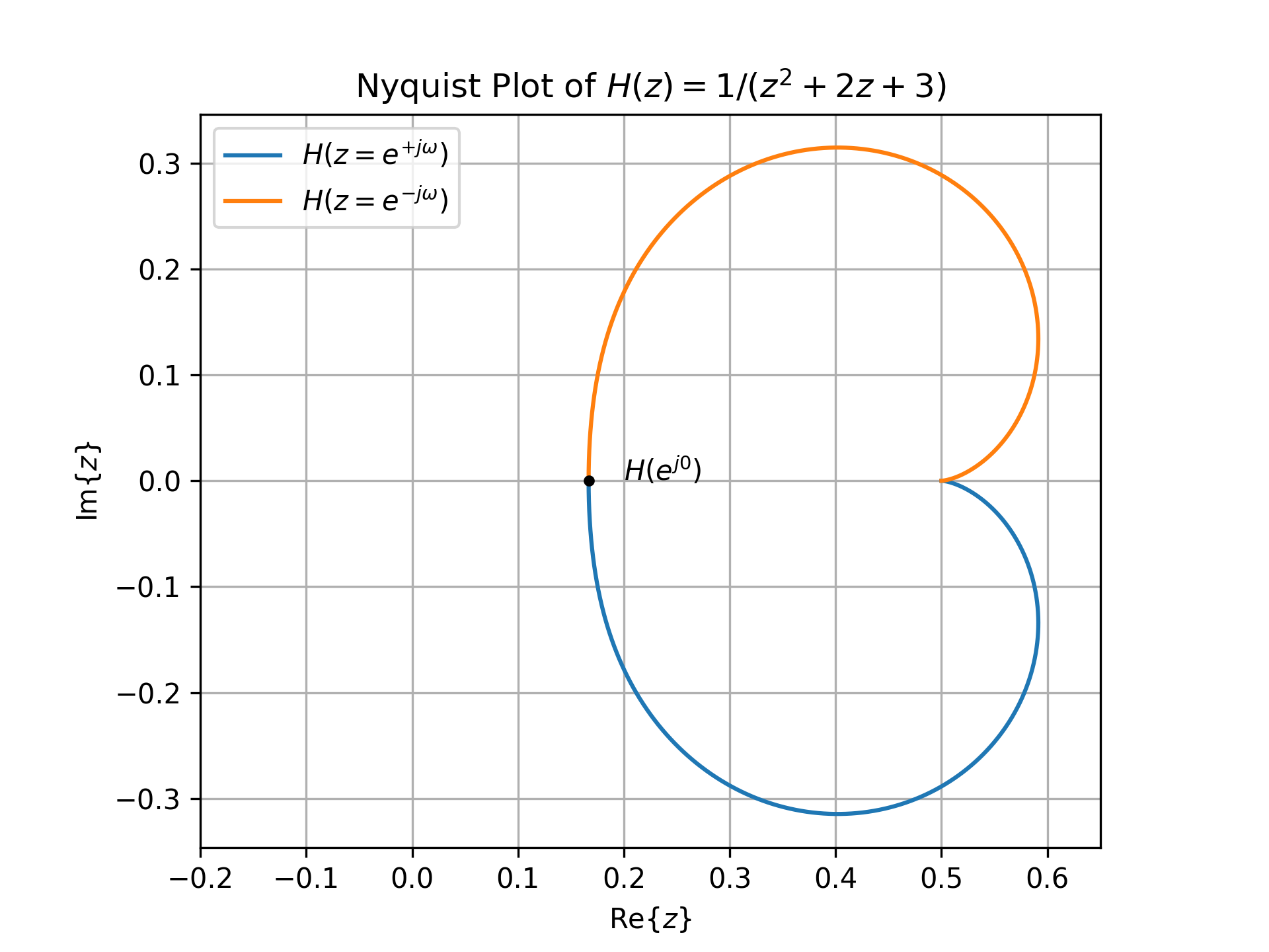
The following example generates the Nyquist plot of the transfer function :math:`H(z) = \frac{1}{z^2 + 2z + 3}` with a sampling time of 0.05 seconds:

from scipy import signal
import matplotlib.pyplot as plt
sys = signal.TransferFunction([1], [1, 2, 3], dt=0.05)  # construct H(z)
w, H = signal.dfreqresp(sys)
fig0, ax0 = plt.subplots()

✓

ax0.plot(H.real, H.imag, label=r"$H(z=e^{+j\omega})$")
ax0.plot(H.real, -H.imag, label=r"$H(z=e^{-j\omega})$")
ax0.set_title(r"Nyquist Plot of $H(z) = 1 / (z^2 + 2z + 3)$")
ax0.set(xlabel=r"$\text{Re}\{z\}$", ylabel=r"$\text{Im}\{z\}$",
        xlim=(-0.2, 0.65), aspect='equal')
ax0.plot(H[0].real, H[0].imag, 'k.')  # mark H(exp(1j*w[0]))
ax0.text(0.2, 0, r"$H(e^{j0})$")

✗

ax0.grid(True)

✓

ax0.legend()

✗

plt.show()

✓

Aliases

scipy.signal.dfreqresp