`scipy.special._orthogonal:laguerre`

source: /scipy/special/_orthogonal.py :731

Signature

def laguerre ( n , monic = False )

Summary

Laguerre polynomial.

Extended Summary

Defined to be the solution of

x \frac{d ^{2}}{d x ^{2}} L_{n} + (1 - x) \frac{d}{d x} L_{n} + n L_{n} = 0;

$L_{n}$ is a polynomial of degree $n$ .

Parameters

n : int: Degree of the polynomial.
monic : bool, optional: If True, scale the leading coefficient to be 1. Default is False.

Returns

L : orthopoly1d: Laguerre Polynomial.

Notes

The polynomials $L_{n}$ are orthogonal over $[0, \infty)$ with weight function $e^{- x}$ .

Examples

The Laguerre polynomials :math:`L_n` are the special case :math:`\alpha = 0` of the generalized Laguerre polynomials :math:`L_n^{(\alpha)}`. Let's verify it on the interval :math:`[-1, 1]`:

import numpy as np
from scipy.special import genlaguerre
from scipy.special import laguerre
x = np.arange(-1.0, 1.0, 0.01)
np.allclose(genlaguerre(3, 0)(x), laguerre(3)(x))

✓

The polynomials :math:`L_n` also satisfy the recurrence relation: .. math:: (n + 1)L_{n+1}(x) = (2n +1 -x)L_n(x) - nL_{n-1}(x) This can be easily checked on :math:`[0, 1]` for :math:`n = 3`:

x = np.arange(0.0, 1.0, 0.01)
np.allclose(4 * laguerre(4)(x),
            (7 - x) * laguerre(3)(x) - 3 * laguerre(2)(x))

✓

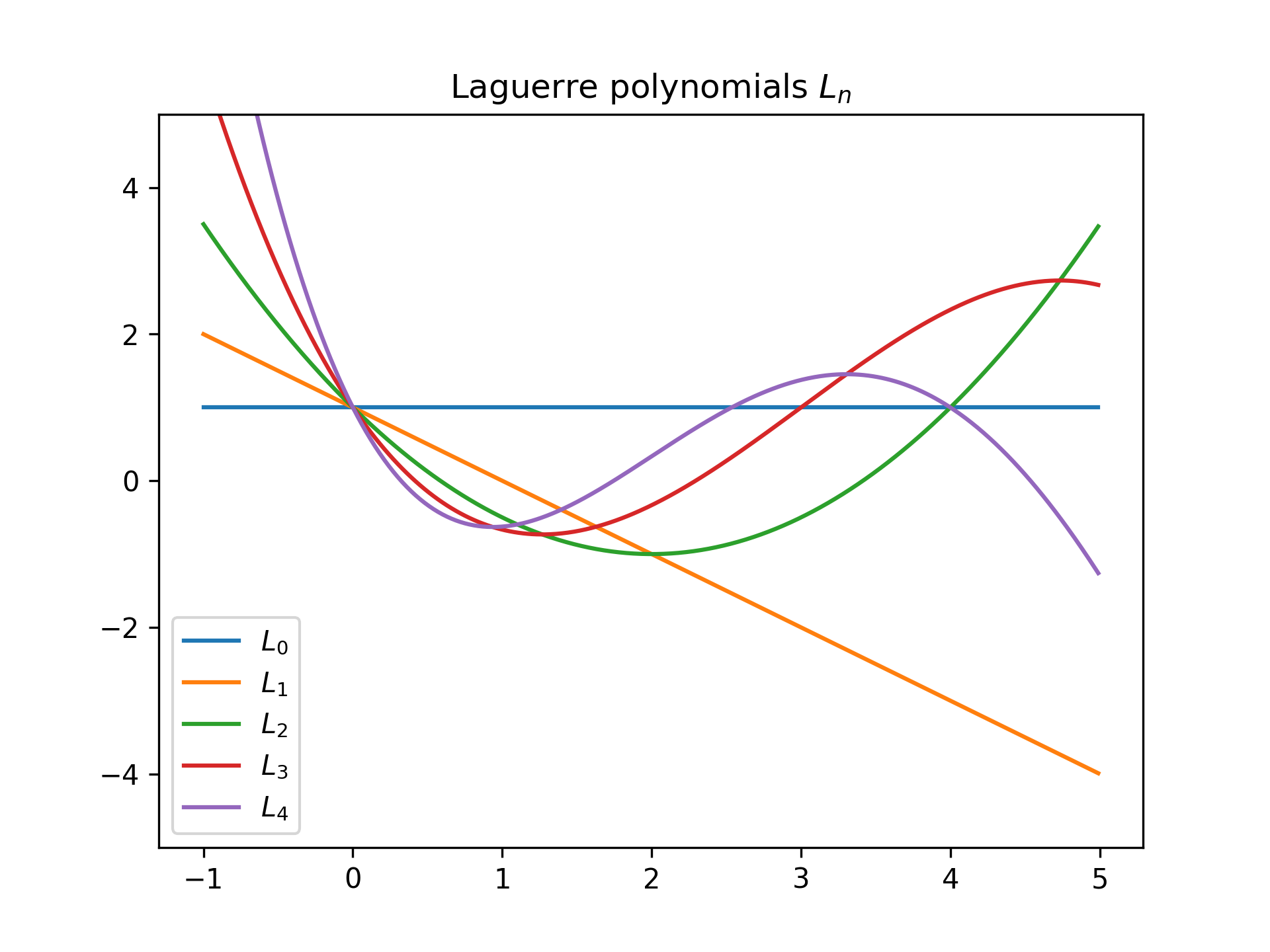
This is the plot of the first few Laguerre polynomials :math:`L_n`:

import matplotlib.pyplot as plt
x = np.arange(-1.0, 5.0, 0.01)
fig, ax = plt.subplots()

✓

ax.set_ylim(-5.0, 5.0)
ax.set_title(r'Laguerre polynomials $L_n$')
for n in np.arange(0, 5):
    ax.plot(x, laguerre(n)(x), label=rf'$L_{n}$')
plt.legend(loc='best')

✗

plt.show()

✓

Aliases

scipy.special.laguerre