bundles / scipy latest / scipy / interpolate / _fitpack2 / SmoothSphereBivariateSpline

class

`scipy.interpolate._fitpack2:SmoothSphereBivariateSpline`

source: /scipy/interpolate/_fitpack2.py :1845

Signature

   class     SmoothSphereBivariateSpline (    theta    ,    phi    ,    r    ,    w    =  None   ,    s    =  0.0   ,    eps    =  1e-16     )

Members

Summary

Smooth bivariate spline approximation in spherical coordinates.

Extended Summary

Parameters

theta, phi, r : array_like: 1-D sequences of data points (order is not important). Coordinates must be given in radians. Theta must lie within the interval [0, pi], and phi must lie within the interval [0, 2pi].
w : array_like, optional: Positive 1-D sequence of weights.
s : float, optional: Positive smoothing factor defined for estimation condition: sum((w(i)*(r(i) - s(theta(i), phi(i))))**2, axis=0) <= s Default s=len(w) which should be a good value if 1/w[i] is an estimate of the standard deviation of r[i].
eps : float, optional: A threshold for determining the effective rank of an over-determined linear system of equations. eps should have a value within the open interval (0, 1), the default is 1e-16.

Notes

For more information, see the FITPACK_ site about this function.

Array API Standard Support

SmoothSphereBivariateSpline is not in-scope for support of Python Array API Standard compatible backends other than NumPy.

See dev-arrayapi for more information.

Examples

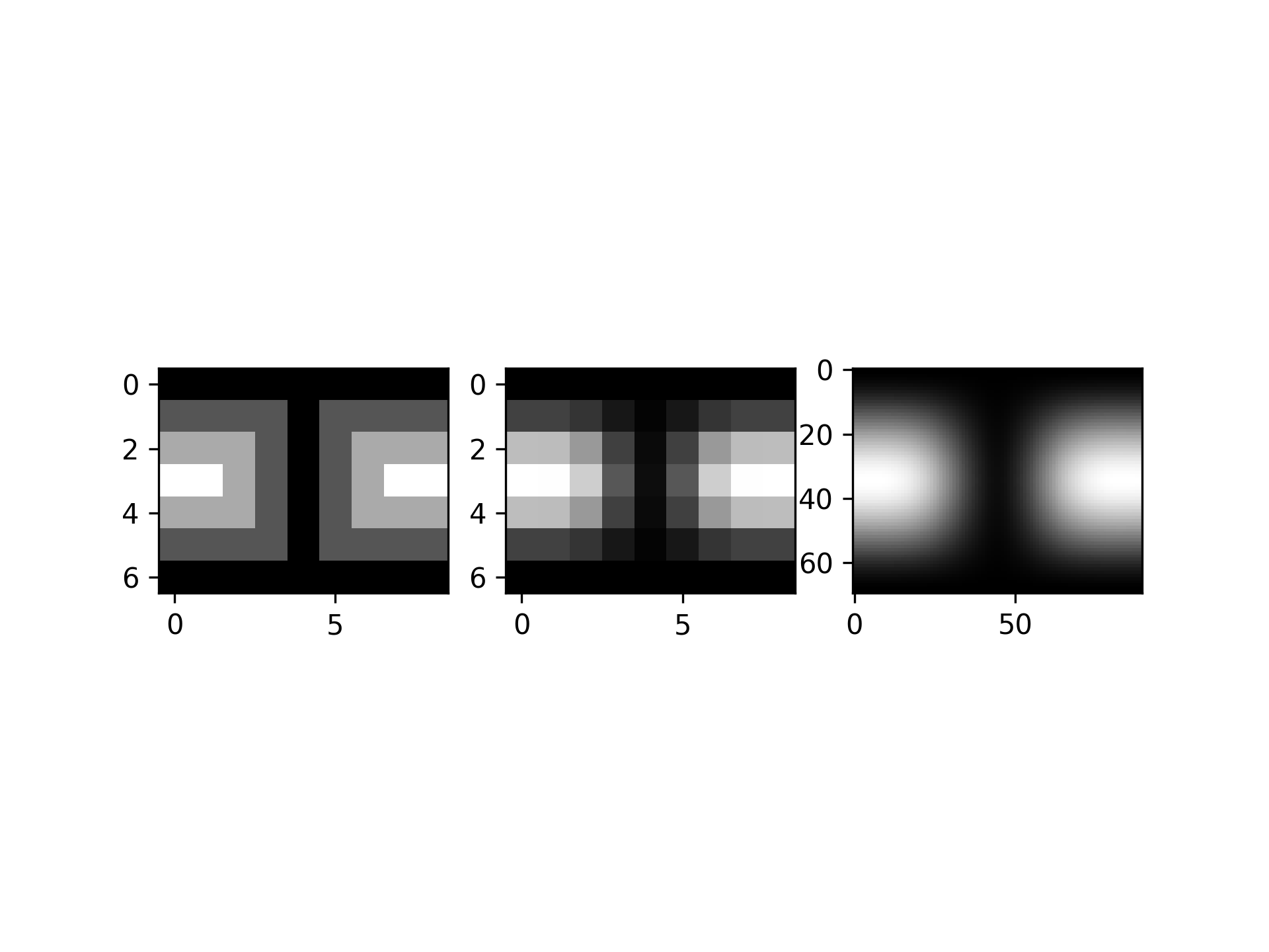
Suppose we have global data on a coarse grid (the input data does not have to be on a grid):

import numpy as np
theta = np.linspace(0., np.pi, 7)
phi = np.linspace(0., 2*np.pi, 9)
data = np.empty((theta.shape[0], phi.shape[0]))
data[:,0], data[0,:], data[-1,:] = 0., 0., 0.
data[1:-1,1], data[1:-1,-1] = 1., 1.
data[1,1:-1], data[-2,1:-1] = 1., 1.
data[2:-2,2], data[2:-2,-2] = 2., 2.
data[2,2:-2], data[-3,2:-2] = 2., 2.
data[3,3:-2] = 3.
data = np.roll(data, 4, 1)

✓

We need to set up the interpolator object

lats, lons = np.meshgrid(theta, phi)
from scipy.interpolate import SmoothSphereBivariateSpline
lut = SmoothSphereBivariateSpline(lats.ravel(), lons.ravel(),
                                  data.T.ravel(), s=3.5)

✓

As a first test, we'll see what the algorithm returns when run on the input coordinates

data_orig = lut(theta, phi)

✓

Finally we interpolate the data to a finer grid

fine_lats = np.linspace(0., np.pi, 70)
fine_lons = np.linspace(0., 2 * np.pi, 90)

✓

data_smth = lut(fine_lats, fine_lons)

✓

import matplotlib.pyplot as plt
fig = plt.figure()
ax1 = fig.add_subplot(131)

✓

ax1.imshow(data, interpolation='nearest')

✗

ax2 = fig.add_subplot(132)

✓

ax2.imshow(data_orig, interpolation='nearest')

✗

ax3 = fig.add_subplot(133)

✓

ax3.imshow(data_smth, interpolation='nearest')

✗

plt.show()

✓

Aliases

scipy.interpolate.SmoothSphereBivariateSpline