bundles / scipy latest / scipy / interpolate / _polyint / BarycentricInterpolator

class

`scipy.interpolate._polyint:BarycentricInterpolator`

source: /scipy/interpolate/_polyint.py :537

Signature

   class     BarycentricInterpolator (    xi    ,    yi    =  None   ,    axis    =  0   ,  * ,     wi    =  None   ,    rng    =  None   ,    random_state    =  None     )

Members

Summary

Barycentric (Lagrange with improved stability) interpolator (C∞ smooth).

Extended Summary

Constructs a polynomial that passes through a given set of points. Allows evaluation of the polynomial and all its derivatives, efficient changing of the y-values to be interpolated, and updating by adding more x- and y-values. For numerical stability, a barycentric representation is used rather than computing the coefficients of the polynomial directly.

Parameters

xi : array_like, shape (npoints, )

1-D array of x-coordinates of the points the polynomial should pass through

yi : array_like, shape (..., npoints, ...), optional

N-D array of y-coordinates of the points the polynomial should pass through. If None, the y values will be supplied later via the set_y method. The length of yi along the interpolation axis must be equal to the length of xi. Use the axis parameter to select correct axis.

axis : int, optional

Axis in the yi array corresponding to the x-coordinate values. Defaults to axis=0.

wi : array_like, optional

The barycentric weights for the chosen interpolation points xi. If absent or None, the weights will be computed from xi (default). This allows for the reuse of the weights wi if several interpolants are being calculated using the same nodes xi, without re-computation. This also allows for computing the weights explicitly for some choices of xi (see notes).

rng : {None, int, `numpy.random.Generator`}, optional

If rng is passed by keyword, types other than numpy.random.Generator are passed to numpy.random.default_rng to instantiate a Generator. If rng is already a Generator instance, then the provided instance is used. Specify rng for repeatable interpolation.

If this argument random_state is passed by keyword, legacy behavior for the argument random_state applies:

If random_state is None (or numpy.random), the numpy.random.RandomState singleton is used.
If random_state is an int, a new RandomState instance is used, seeded with random_state.
If random_state is already a Generator or RandomState instance then that instance is used.

Notes

This method is a variant of Lagrange polynomial interpolation ^[1] based on ^[2]. Instead of using Lagrange's or Newton's formula, the polynomial is represented by the barycentric formula

p (x) = \frac{\sum _{i = 1}^{m} w _{i} y _{i} / ( x - x _{i} )}{\sum _{i = 1}^{m} w _{i} / ( x - x _{i} )},

where $w_{i}$ are the barycentric weights computed with the general formula

w_{i} = k \neq = i \prod x_{i} - x_{k}^{- 1} .

This is the same barycentric form used by AAA and FloaterHormannInterpolator. However, in contrast, the weights $w_{i}$ are defined such that $p (x)$ is a polynomial rather than a rational function.

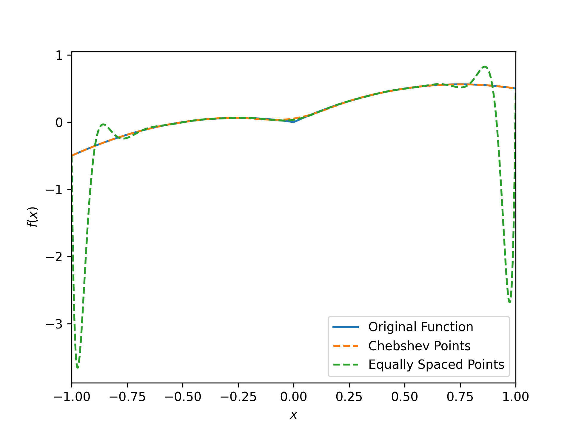
The barycentric representation avoids many of the problems associated with polynomial interpolation caused by floating-point arithmetic. However, it does not avoid issues that are intrinsic to polynomial interpolation. Namely, if the x-coordinates are equally spaced, then the weights can be computed explicitly using the formula from ^[2]

w_{i} = (- 1)^{i} (i n),

where $n$ is the number of x-coordinates. As noted in ^[2], this means that for large $n$ the weights vary by exponentially large factors, leading to the Runge phenomenon.

To avoid this ill-conditioning, the x-coordinates should be clustered at the endpoints of the interval. An excellent choice of points on the interval $[a, b]$ are Chebyshev points of the second kind

x_{i} = \frac{a + b}{2} + \frac{a - b}{2} cos (iπ / n) .

in which case the weights can be computed explicitly as

w_{i} = {(- 1)^{i} /2 (- 1)^{i} i = 0, n otherwise .

See ^[2] for more infomation. Note that for large $n$ , computing the weights explicitly (see examples) will be faster than the generic formula.

Examples

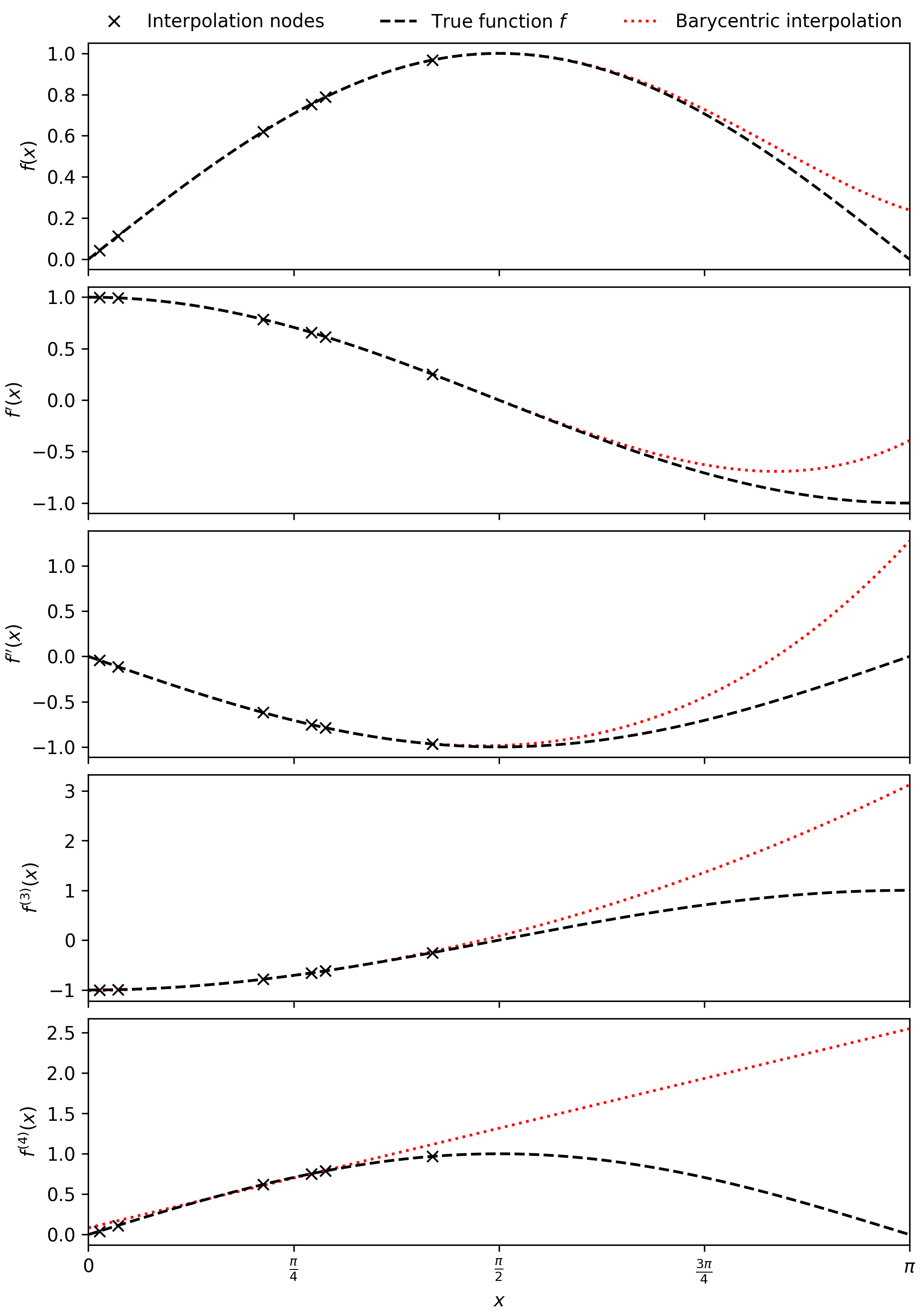
To produce a quintic barycentric interpolant approximating the function :math:`\sin x`, and its first four derivatives, using six randomly-spaced nodes in :math:`(0, \pi/2)`:

import numpy as np
import matplotlib.pyplot as plt
from scipy.interpolate import BarycentricInterpolator
rng = np.random.default_rng()
xi = rng.random(6) * np.pi/2
f, f_d1, f_d2, f_d3, f_d4 = np.sin, np.cos, lambda x: -np.sin(x), lambda x: -np.cos(x), np.sin
P = BarycentricInterpolator(xi, f(xi), random_state=rng)
fig, axs = plt.subplots(5, 1, sharex=True, layout='constrained', figsize=(7,10))
x = np.linspace(0, np.pi, 100)

✓

axs[0].plot(x, P(x), 'r:', x, f(x), 'k--', xi, f(xi), 'xk')
axs[1].plot(x, P.derivative(x), 'r:', x, f_d1(x), 'k--', xi, f_d1(xi), 'xk')
axs[2].plot(x, P.derivative(x, 2), 'r:', x, f_d2(x), 'k--', xi, f_d2(xi), 'xk')
axs[3].plot(x, P.derivative(x, 3), 'r:', x, f_d3(x), 'k--', xi, f_d3(xi), 'xk')
axs[4].plot(x, P.derivative(x, 4), 'r:', x, f_d4(x), 'k--', xi, f_d4(xi), 'xk')
axs[0].set_xlim(0, np.pi)
axs[4].set_xlabel(r"$x$")
axs[4].set_xticks([i * np.pi / 4 for i in range(5)],
                  ["0", r"$\frac{\pi}{4}$", r"$\frac{\pi}{2}$", r"$\frac{3\pi}{4}$", r"$\pi$"])
for ax, label in zip(axs, ("$f(x)$", "$f'(x)$", "$f''(x)$", "$f^{(3)}(x)$", "$f^{(4)}(x)$")):
    ax.set_ylabel(label)

✗

labels = ['Interpolation nodes', 'True function $f$', 'Barycentric interpolation']

✓

axs[0].legend(axs[0].get_lines()[::-1], labels, bbox_to_anchor=(0., 1.02, 1., .102),
              loc='lower left', ncols=3, mode="expand", borderaxespad=0., frameon=False)

✗

plt.show()

✓

Next, we show how using Chebyshev points of the second kind avoids the Runge phenomenon. In this example, we also compute the weights explicitly.

n = 20
def f(x): return np.abs(x) + 0.5*x - x**2
i = np.arange(n)
x_cheb = np.cos(i*np.pi/(n - 1))  # Chebyshev points on [-1, 1]
w_i_cheb = (-1.)**i  # Explicit formula for weights of Chebyshev points
w_i_cheb[[0, -1]] /= 2
p_cheb = BarycentricInterpolator(x_cheb, f(x_cheb), wi=w_i_cheb)
x_equi = np.linspace(-1, 1, n)
p_equi = BarycentricInterpolator(x_equi, f(x_equi))
xx = np.linspace(-1, 1, 1000)
fig, ax = plt.subplots()

✓

ax.plot(xx, f(xx), label="Original Function")
ax.plot(xx, p_cheb(xx), "--", label="Chebshev Points")
ax.plot(xx, p_equi(xx), "--", label="Equally Spaced Points")
ax.set(xlabel="$x$", ylabel="$f(x)$", xlim=[-1, 1])
ax.legend()

✗

plt.show()

✓

Aliases

scipy.interpolate.BarycentricInterpolator